RectangularLocations Command
This section assumes you are very familiar with the concepts, terms and ideas for protograf as presented in the Basic Concepts , that you understand all of the Additional Concepts and that you’ve created some basic scripts of your own using the Core Shapes.
This is part of the set of commands used for Layouts, that are used in conjunction with the Layout command.
Overview
The RectangularLocations() command defines an ordered series
of row and column locations that create a rectangular grid.
The x- and y-values of these rows and columns are then used to set the centres of the shapes that can be placed there using the Layout() command.
The centres of the rows and columns themselves are not drawn — if needed you can use the debug property to display them (see Example 10. Debug below).
Apart from the RectangularLocations() command described here,
there are also these other commands which allow you to layout
elements in a more repetitive or regular way within a page:
Usage
RectangularLocations() creates a “virtual” grid that always has the
first row and first column in the upper-left corner and the last row and last
column in the lower-right corner.
The command accepts the following properties:
cols - this is the number of locations in the horizontal direction; this defaults to 2
rows - this is the number of locations in the vertical direction; this defaults to 2
interval - this is horizontal distance between columns, as well as the vertical distance between rows, in the grid; defaults to
1cminterval_x - this is horizontal distance between the centres of the columns in the grid; defaults to interval
interval_y - this is vertical distance between the centres of the rows in the gridl defaults to interval
direction - this is the compass direction of the line of travel when creating the row and column layout; the default is e(ast).
start - this is the initial corner, defined a secondary compass direction, from where the grid is initially drawn; values can be ne, nw, se, and sw, the default i.e. the lower-left corner
pattern - this is the way in which the grid is drawn; the default behaviour is to draw each row, and then move across all columns in a regular line; but the setting can also be:
snaking - which means the direction is reversed across each row
outer - which means only the locations in the outer-most edge of the grid are created
Note
Bear in mind that the RectangularLocations() command is designed
to work in conjunction with a Layout() command
which accepts, as its first property, the name assigned to the grid.
Properties
All examples below make use of a common Circle shape (assigned to
the name a_circle) defined as:
a_circle = circle(
    x=0, y=0, diameter=1.0,
    label="{{sequence}}//{{col}}-{{row}}", label_size=6)
In these examples, the placeholder names {{sequence}}, {{col}}
and {{row}} will be replaced, in the label for the Circle, by the
values for the row and column in which that circle is placed, as well as
by the sequence value - or order number - in which that Circle gets drawn,
starting from zero.
Hint
To start the sequence from any other number, simply add or subtract that
number from the sequence, for example, {{sequence + 1}} or
{{sequence - 10}}.
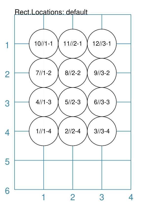
Example 1. Rows and Columns
|
This example shows the design constructed using the following values for the shapes’ properties. rect = RectangularLocations(
cols=3, rows=4)
Layout(rect, shapes=[a_circle])
As can be seen the sequence starts, by default, in the lower-left; and increases from left to right and then from bottom to top. The column and row numbers (which follow next to the // in the
label) show that the topmost row is |
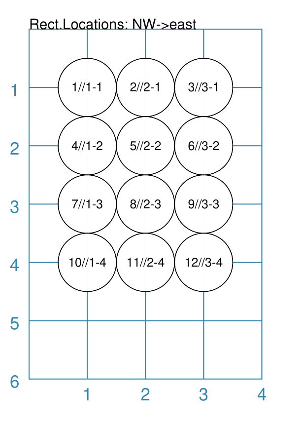
Example 2. Start and Direction
|
This example shows the design constructed using the following values for the shapes’ properties. rect = RectangularLocations(
cols=3, rows=4,
start="NW", direction="east")
Layout(rect, shapes=[a_circle])
Here the sequence starts in the top-left / northwest (“NW”) corner, and then flows to the right (“east”) and down. |
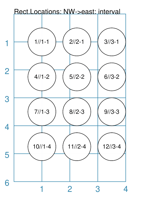
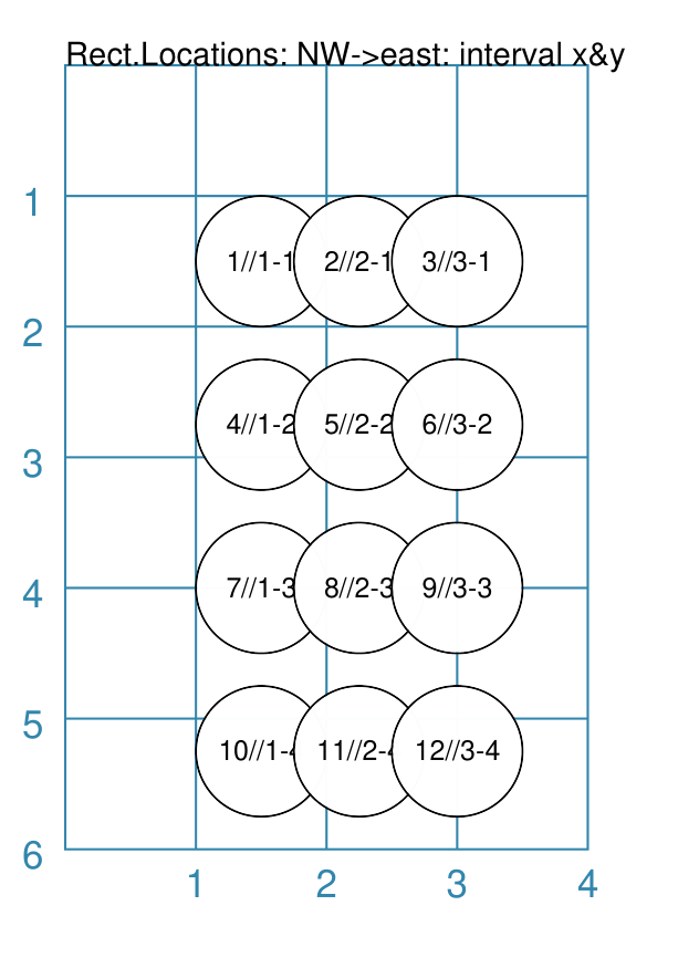
Example 3. Row and Column Interval
|
This example shows the design constructed using the following values for the shapes’ properties. rect = RectangularLocations(
cols=3, rows=4, start="NW", direction="east",
interval=1.25)
Layout(rect, shapes=[a_circle])
Here the sequence starts in the top-left / northwest (“NW”) corner, and then flows to the right (“east”) and down. The interval property adds spacing in both x- and y-directions. |
|
This example shows the design constructed using the following values for the shapes’ properties. rect = RectangularLocations(
cols=3, rows=4, start="NW", direction="east",
x=1.5, y=1.5,
interval_y=1.25, interval_x=0.75)
Layout(rect, shapes=[a_circle])
The x-interval property adds spacing in the x-direction, which is less than the y-interval property spacing in the y-direction. |
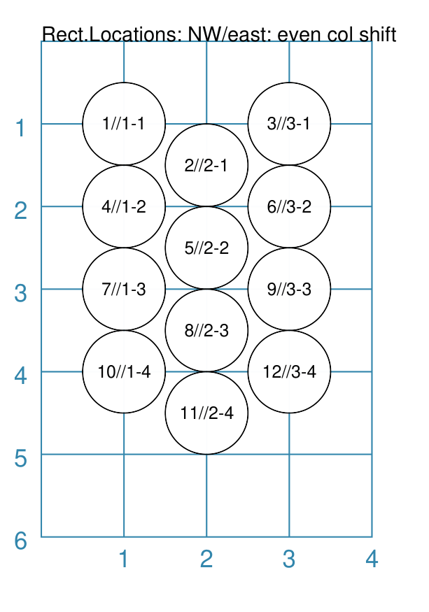
Example 4. Row and Column Offset
|
This example shows the design constructed using the following values for the shapes’ properties. rect = RectangularLocations(
cols=3, rows=4,
start="NW", direction="east",
col_even=0.5)
Layout(rect, shapes=[a_circle])
The col_even adds a positive value to every even column, making these shift downwards relative to the odd columns. Setting a value for col_odd would have the opposite effect. |
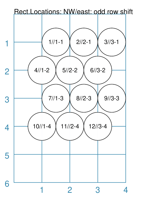
|
This example shows the design constructed using the following values for the shapes’ properties. rect = RectangularLocations(
cols=3, rows=4,
start="NW", direction="east",
row_odd=0.5)
Layout(rect, shapes=[a_circle])
The row_odd adds a positive value to every odd row, making these shift rightwards relative to the even rows. Setting a value for row_even would have the opposite effect. |
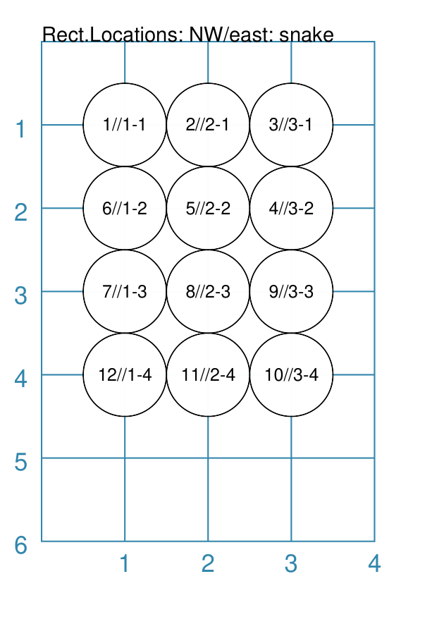
Example 5. Snaking
|
This example shows the design constructed using the following values for the shapes’ properties. rect = RectangularLocations(
cols=3, rows=4,
start="NW", direction="east",
pattern="snake")
Layout(rect, shapes=[a_circle])
The |
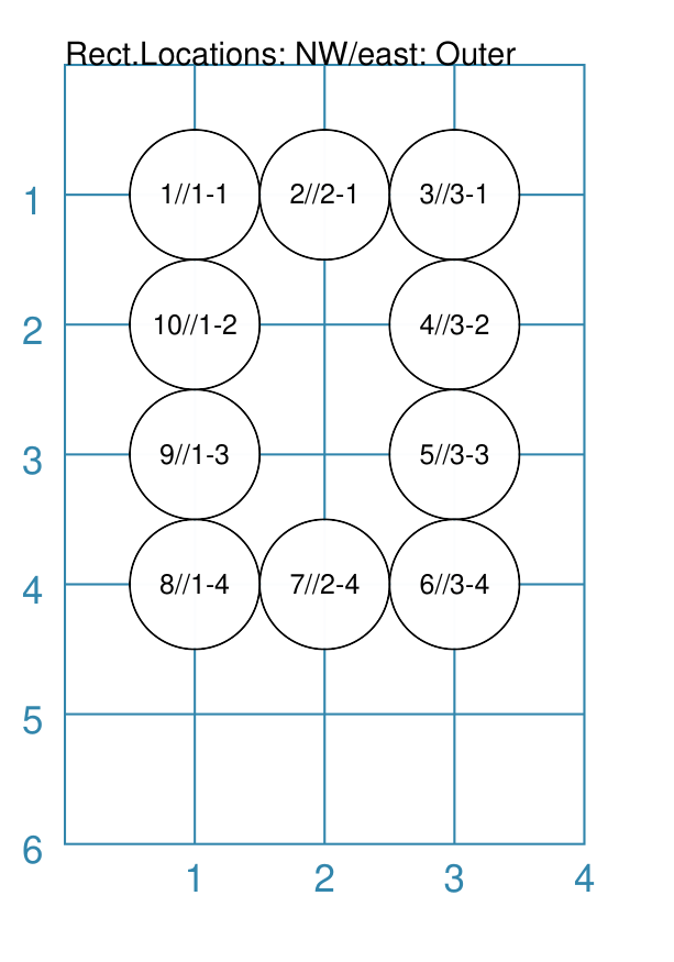
Example 6. Outer Edge
|
This example shows the design constructed using the following values for the shapes’ properties. rect = RectangularLocations(
cols=3, rows=4,
start="NW", direction="east",
pattern="outer")
Layout(rect, shapes=[a_circle])
The The sequence starts off So, the combination of the start property and the initial direction property determine how an outer sequence proceeds. |
Note
The examples below all make use of some Common elements:
is_common = Common(label="{{sequence}}")
rct_common = Common(
    height=0.5, width=0.5,
    label_size=5, points=[('s', 0.1)])
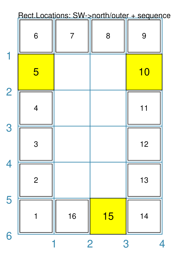
Example 6a. Outer Edge - Shapes
|
This example shows the design constructed using the following values for the shapes’ properties. is_common = Common(label="{{sequence + 1}}")
sqr = square(common=is_common, side=0.9,
label_size=6)
sqr5 = square(common=is_common, side=1.0,
label_size=8, fill="yellow")
rect = RectangularLocations(
x=0.5, y=0.5,
cols=4, rows=6, interval=1,
start="SW", direction="north",
pattern="outer")
Layout(rect, shapes=[sqr]*4 + [sqr5] )
This example shows how to provide copies of different shapes that must be drawn. Using the Similarly, using Both In summary, the final list of shapes becomes:
This notation can also be used if the approach shown in the example is too confusing! As before, the |
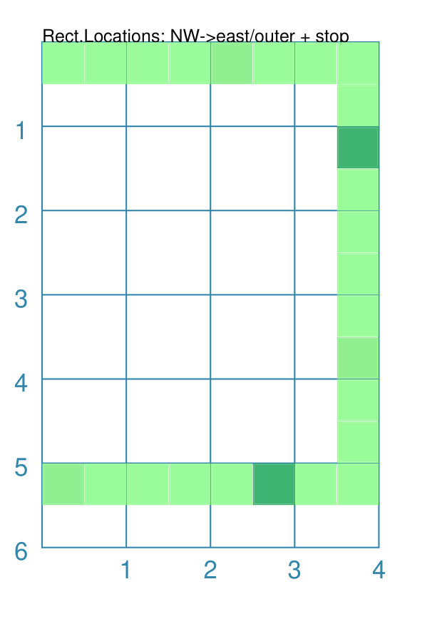
Example 6b. Outer Edge - Stop and Start
|
This example shows the design constructed using the following values for the shapes’ properties. rct_small = Common(label_size=5, side=0.48)
rct1 = square(
common=rct_small,
fill_stroke="palegreen")
rct5 = square(
common=rct_small,
fill_stroke="lightgreen")
rct10 = square(
common=rct_small,
fill_stroke="mediumseagreen")
rect = RectangularLocations(
x=0.25, y=0.25,
cols=8, rows=11, interval=0.5
start="NW", direction="east",
pattern="outer",
stop=26)
Layout(rect, shapes=[rct1]*4 + [rct5] + [rct1]*4 + [rct10])
This example shows how by providing a value of The setting and drawing of shapes is as per the previous example. Note that it does not matter how many locations will be used; when all shapes in the list have been processed the cycle will start again with the first. |
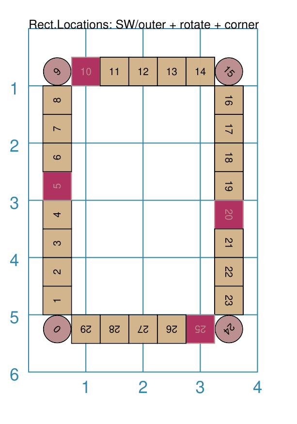
Example 6c. Outer Edge - Rotation
|
This example shows the design constructed using the following values for the shapes’ properties. rct_common = Common(
label_size=5, points=[('s', 0.1)],
height=0.5, width=0.5)
circ = circle(
label="{{sequence}}",
label_size=5, radius=0.26, fill="rosybrown")
rct2 = rectangle(
common=rct_common, label="{{sequence}}",
fill="tan")
rct3 = rectangle(
common=rct_common, label="{{sequence}}",
fill="maroon", stroke="rosybrown")
locs = RectangularLocations(
x=0.5, y=0.75, cols=7, rows=10, interval=0.5,
start="SW", direction="north", pattern="outer")
Layout(
locs,
shapes=[rct3] + [rct2]*4,
rotations=[
("1", 135),
("2-9", 90),
("10", 45),
("16", -45),
("17-24", 270),
("25", 225),
("26-30", 180)
],
corners=[('*',circ)])
Labels are created by use of the The rotations property references specific sequence values in a list of
sets of values; for example, The rotations property sequence value is the original one; not the one being displayed! The corners settings allows the corner elements to be replaced by those
appearing in this list - in this case the use of |
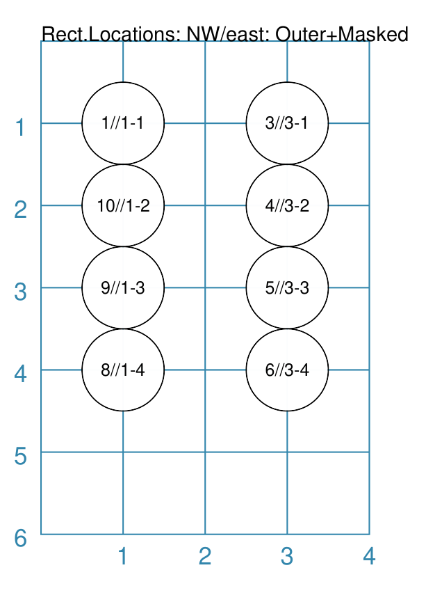
Example 7. Masked
|
This example shows the design constructed using the following values for the shapes’ properties. rect = RectangularLocations(
cols=3, rows=4, start="NW",
direction="east",
pattern="outer")
Layout(rect, shapes=[a_circle],
masked=[2,7])
The masked property means that two of the shapes — corresponding
to sequence numbers |
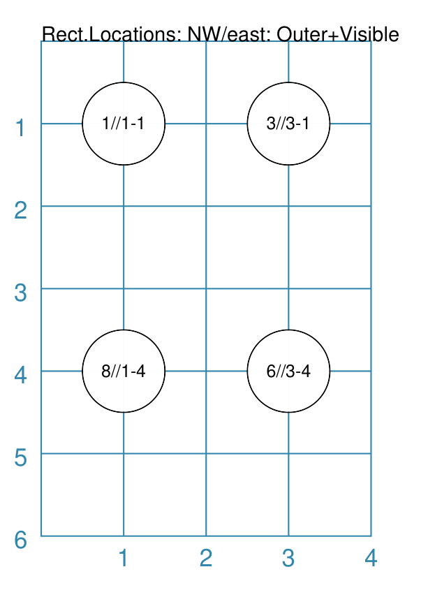
Example 8. Visible
|
This example shows the design constructed using the following values for the shapes’ properties. rect = RectangularLocations(
cols=3, rows=4, start="NW",
direction="east",
pattern="outer")
Layout(rect, shapes=[a_circle],
visible=[1,3,6,8])
The visible property means that only those shapes — corresponding
to sequence numbers |
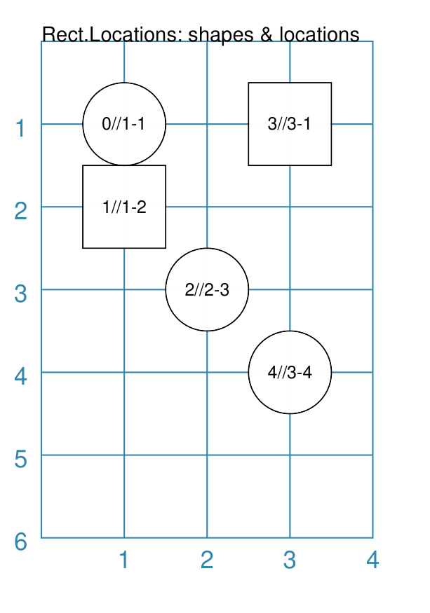
Example 9. Locations Setting
|
This example shows the design constructed using the following values for the shapes’ properties. rect = RectangularLocations(cols=3, rows=4)
Layout(
rect,
shapes=[
a_circle,
rectangle(
label="{{sequence}}//{{col}}-{{row}}",
label_size=6)],
locations=[(1,2), (2,3), (3,1), (1,1), (3,4)])
The shapes are allocated to the list of locations provided. Each location is identified by its pair of The shape allocation cycles through the list of shapes provided; in this case the Circle and Rectangle. |
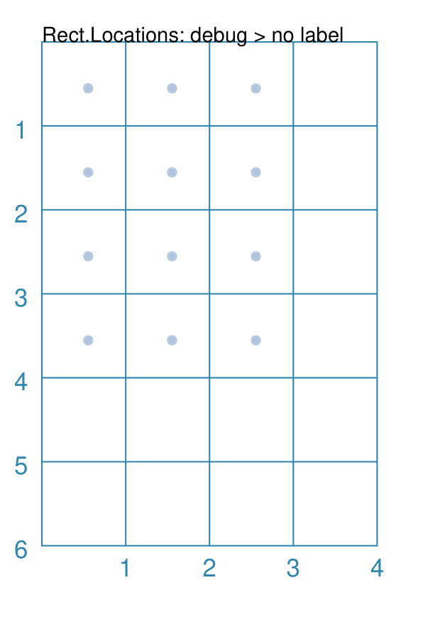
Example 10. Debug
|
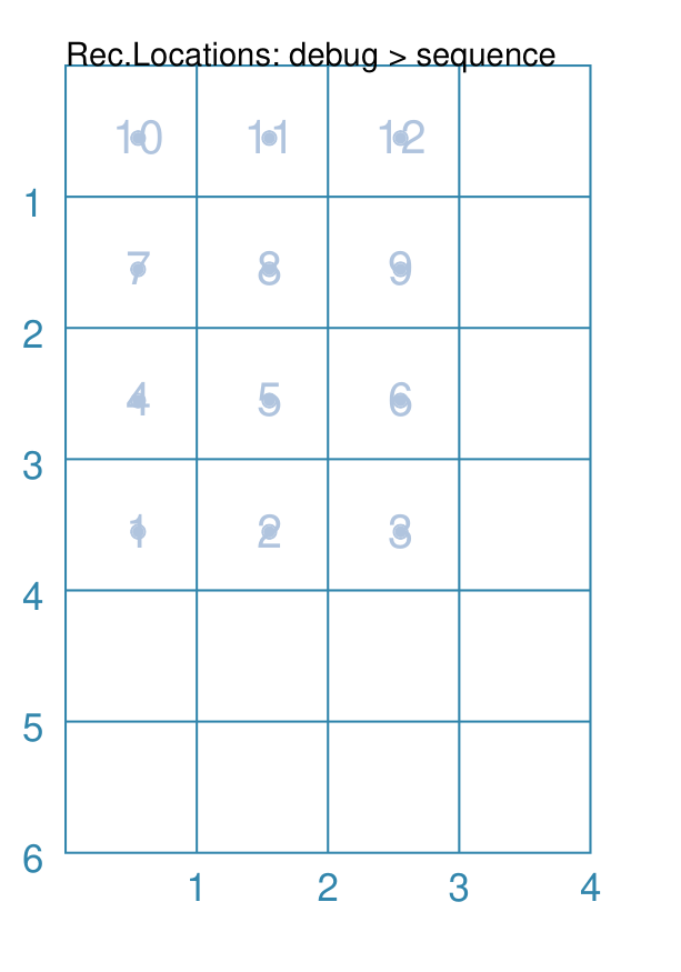
This example shows the design constructed using the following values for the shapes’ properties. rect = RectangularLocations(
cols=3, rows=4, x=0.5, y=0.5)
Layout(rect, debug='none')
In this case, setting the debug property to This is useful to visualise the centre positions to see where shapes could be drawn. |
|
This example shows the design constructed using the following values for the shapes’ properties. rect = RectangularLocations(
cols=3, rows=4, x=0.5, y=0.5)
Layout(rect, debug='sequence')
In this case, setting the debug property to This is useful to visualise the order in which shapes would be drawn at the locations. |
|
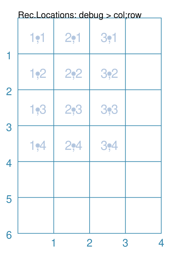
This example shows the design constructed using the following values for the shapes’ properties. rect = RectangularLocations(
cols=3, rows=4, x=0.5, y=0.5)
Layout(rect, debug='colrow')
In this case, setting the debug property to This is useful to visualise the identity of each location; for example, if you needed to make any of these locations visible or masked. |
Example 11. Gridlines - Orthogonal
|
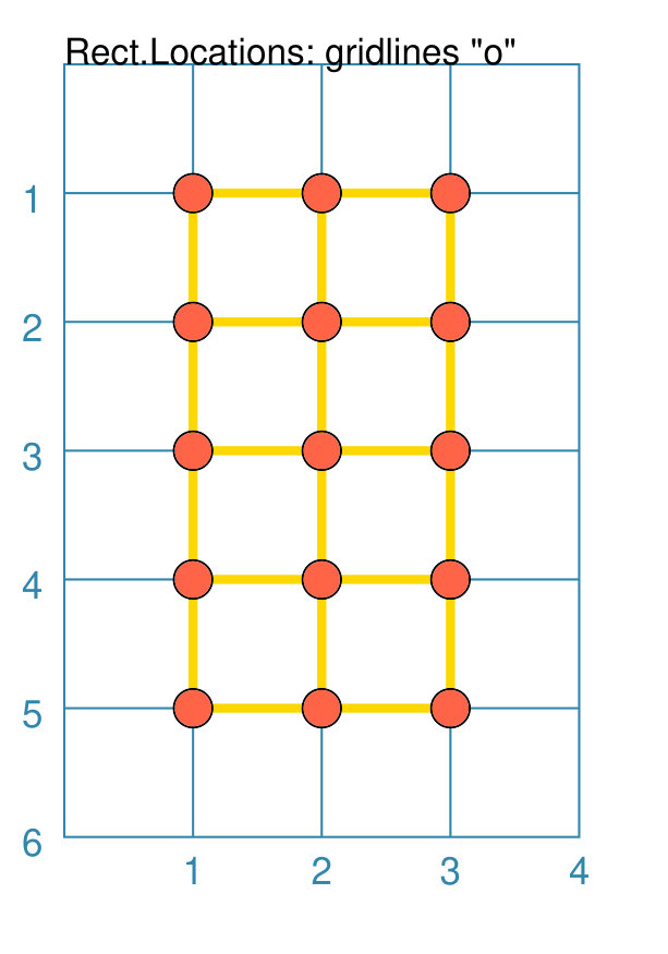
This example shows the design constructed using the following values for the shapes’ properties. small_circle = circle(
radius=0.15,
fill="tomato")
rct = RectangularLocations(
cols=3, rows=5,
start="NE",
direction="west")
Layout(
rct,
gridlines='o',
gridlines_stroke="gold",
gridlines_stroke_width=2,
shapes=[small_circle])
Here, the grid itself is displayed — it is always drawn first before any shapes. The outline of the grid is always drawn. The key prefix is gridlines and the value assigned to it will
determine in which direction, or directions, the gridlines are drawn;
in this case, all The usual customisation settings are possible for the gridlines; color, thickness, etc. |
Example 12. Gridlines - Diagonal
|
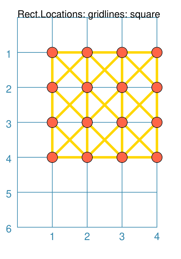
This example shows the design constructed using the following values for the shapes’ properties. small_circle = circle(
radius=0.15,
fill="tomato")
rct = RectangularLocations(
cols=4, rows=4,
start="NE",
direction="west")
Layout(
rct,
gridlines='d n',
gridlines_stroke="gold",
gridlines_stroke_width=2,
shapes=[small_circle])
Here, the grid itself is displayed — it is always drawn first before any shapes. The outline of the grid is always drawn. The key prefix is gridlines and the value assigned to it will
determine in which direction, or directions, the gridlines are drawn;
in this case, all The usual customisation settings are possible for the gridlines; color, thickness, etc. |
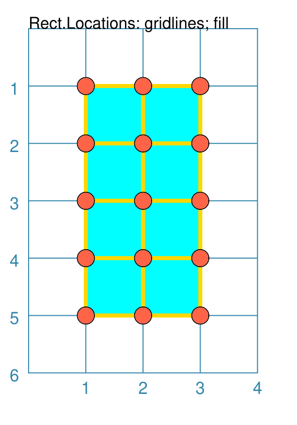
Example 13. Gridlines - Fill
|
This example shows the design constructed using the following values for the shapes’ properties. small_circle = circle(
radius=0.15,
fill="tomato")
rct = RectangularLocations(
cols=3, rows=5,
start="NE",
direction="west")
Layout(
rct,
gridlines='*',
gridlines_fill="aqua",
gridlines_stroke="gold",
gridlines_stroke_width=2,
shapes=[small_circle])
Here, the grid itself is displayed — it is always drawn first before any shapes. The outline of the grid is always drawn. If the gridlines_fill property is assigned a color, then the grid will be filled with that color before any gridlines are drawn. The key prefix is gridlines and the value assigned to it will
determine in which direction, or directions, the gridlines are drawn;
in this case, because of the The usual customisation settings are possible for the gridlines; color, thickness, etc. Note Although gridlines could be drawn in all directions, in this case they will not be because the grid is rectangular — only square shaped grids will have diagonal lines drawn for them. |
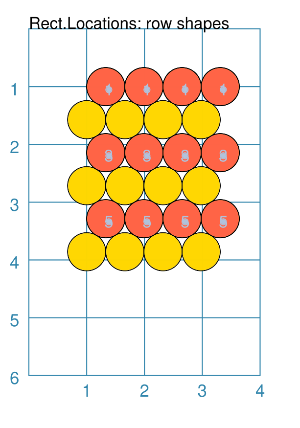
Example 14. Shapes - by Rows
|
This example shows the shape constructed using differing values for its properties. rct = RectangularLocations(
facing='north',
y=1, x=1,
side=.66,
cols=4, rows=6)
Layout(
rct,
shapes=[gold_circle])
Layout(
rct,
rows=[1, 3, 5],
shapes=[red_circle],
debug='c')
Here, two sets of circles are drawn onto the diamond grid. The first set — the The second set — the The debug value in the red circles shows the row number (in order). |
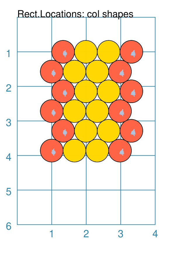
Example 15. Shapes - by Columns
|
This example shows the shape constructed using differing values for its properties. rct = RectangularLocations(
facing='north',
y=1, x=1,
side=.66,
cols=4, rows=6)
Layout(
rct,
shapes=[gold_circle])
Layout(
rct,
cols=[1, 4],
shapes=[red_circle],
debug='c')
Here, two sets of circles are drawn onto the diamond grid. The first set — the The second set — the The debug value in the red circles shows the column number (in order). |