Hexagonal Grids
This section assumes you are very familiar with the concepts, terms and ideas for protograf as presented in the Basic Concepts , that you understand all of the Additional Concepts and that you’ve created some basic scripts of your own using the Core Shapes.
Overview
Hexagonal grids are now widely used in the table top gaming industry.
They are particularly suitable in providing an overlay for maps and have been used for decades in war games and role playing games, but can also act as grids or tiles in regular board games.
Some practical examples of these grids are shown in the section with both commercial and abstract boards.
You should have already seen how a single Hexagon and a basic grid of Hexagons are created using defaults. You should also have seen how a single hexagon can be further enhanced as a Customised Hexagon Shape.
Rectangular Hexagonal Grid
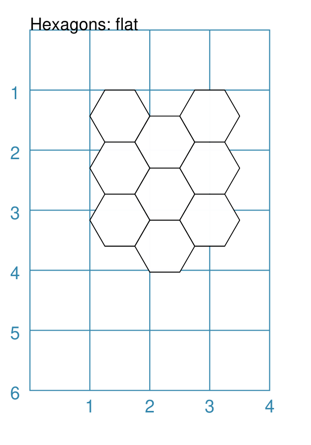
The basic hexagonal grid is laid out in a rectangular fashion. It can be customised in a number of ways.
Rows and Columns
|
This example shows a grid constructed using the command: Hexagons(
side=0.5,
x=1, y=1,
rows=3, cols=3
)
It has the following properties that differ from the defaults:
|
|
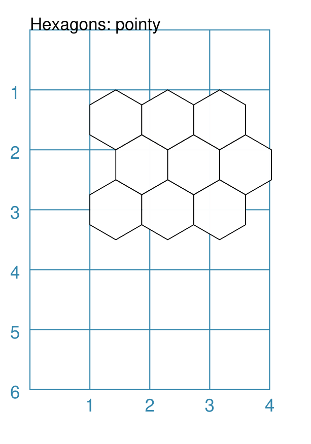
This example shows a grid constructed using the command: Hexagons(
side=0.5,
x=1, y=1,
rows=3, cols=3,
orientation="pointy"
)
It has the following properties that differ from the defaults:
|
Coordinates
Every location in a grid has a row and column number — these are not, by default, displayed on the grid; but they are needed in some cases; for example, to support grid references for a wargame map.
The coordinate system starts at the top-left of the grid; the column is, by default, the first value (the “x” location) and the row is the second value (the “y” location).
The coordinates can be displayed using either letters (upper or lowercase) or
numbers (the default behaviour). A separator may be specified to help
visualise, or differentiate, the row versus the column value. For numeric
coordinates, numbers have a “zero padding”; so 1 is displayed as 01.
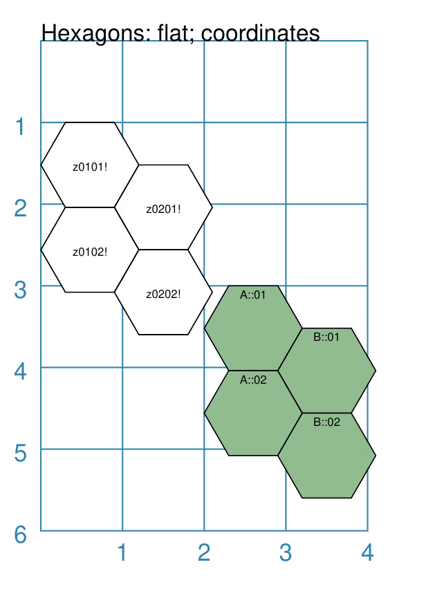
The coordinates can also be displayed in various positions within the hexagon.
Most coordinate property names are prefixed with coord_.
|
This example shows grids constructed using the commands: Hexagons(
side=0.6,
x=0, y=0,
rows=2, cols=2,
coord_elevation="middle",
coord_prefix='z',
coord_suffix='!',
)
Hexagons(
side=0.6,
x=2, y=3,
rows=2, cols=2,
fill="darkseagreen",
coord_elevation="top",
coord_type_x="upper",
coord_separator='::',
)
Each has the following properties that differ from the defaults:
The white grid also has:
The green grid also has:
|
|
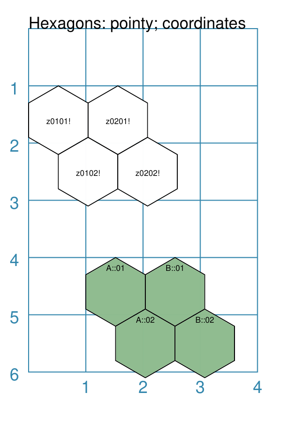
This example shows grids constructed using the commands: Hexagons(
side=0.6,
x=0, y=1,
rows=2, cols=2,
orientation="pointy",
fill="white",
coord_elevation="middle",
coord_prefix='z',
coord_suffix='!',
)
Hexagons(
side=0.6,
x=1, y=4,
rows=2, cols=2,
orientation="pointy",
fill="darkseagreen",
coord_elevation="top",
coord_type_x="upper",
coord_separator='::',
)
Each has the following properties that differ from the defaults:
The white grid also has:
The green grid also has:
|
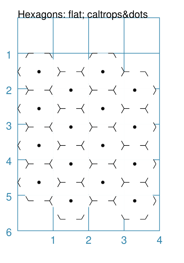
Caltrops
Caltrops is a term when the point at which three hexagons meet is drawn by a set of three small lines; these replace the normal edge of the hexagon.
|
This example shows a grid constructed using the command: Hexagons(
side=0.6,
x=0, y=1,
rows=3, cols=3,
dot=0.04,
caltrops=0.15,
)
It has the following properties that differ from the defaults:
|
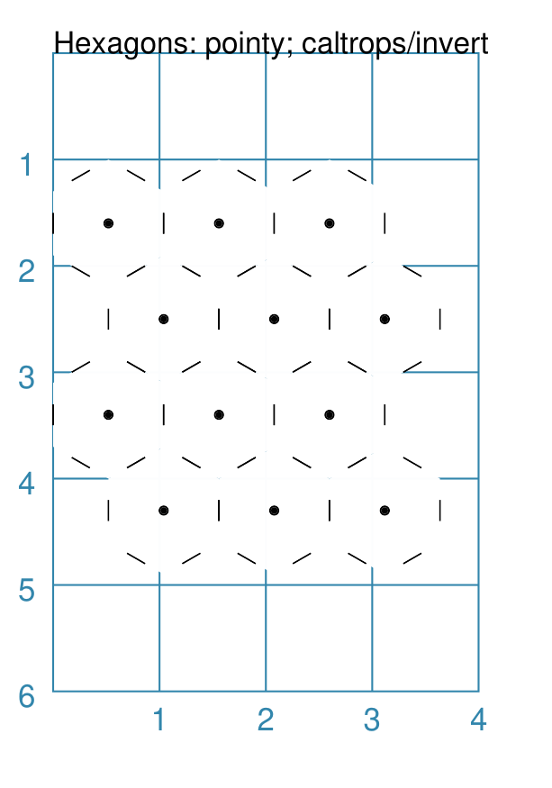
|
This example shows a grid constructed using the command: Hexagons(
side=0.6,
x=0, y=1,
rows=3, cols=3,
orientation="pointy",
dot=0.04,
caltrops=0.2,
caltrops_invert=True,
)
It has the following properties that differ from the defaults:
|
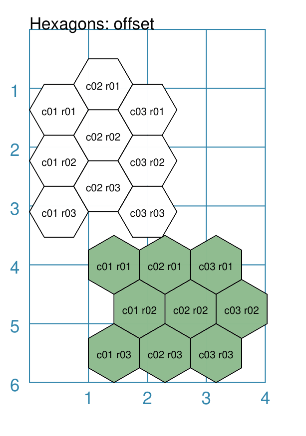
Offset
|
This example shows grids constructed using the commands: Hexagons(
side=0.5,
x=0, y=0.5,
rows=3, cols=3,
hex_offset="even",
coord_elevation="middle",
coord_font_size=5,
coord_separator=' r',
coord_prefix='c',
)
Hexagons(
side=0.5,
x=1, y=3.5,
rows=3, cols=3,
hex_offset="even",
orientation="pointy",
fill="darkseagreen",
coord_elevation="middle",
coord_font_size=5,
coord_separator=' r',
coord_prefix='c',
)
Each has the following properties that differ from the defaults:
|
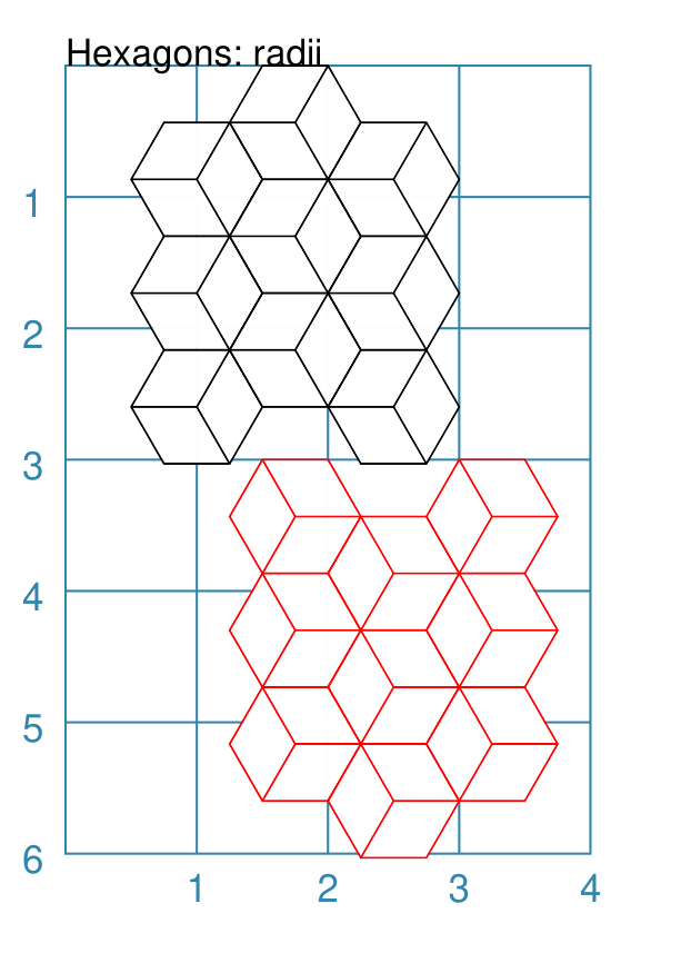
Radii
|
This example shows grids constructed using the commands: Hexagons(
side=0.5,
x=0.5, y=0,
rows=3, cols=3,
hex_offset="odd",
radii="w ne se",
)
Hexagons(
side=0.5,
x=1.25, y=3,
rows=3, cols=3,
stroke="red",
radii_stroke="red",
hex_offset="even",
radii="e nw sw",
)
Each has the following properties that differ from the defaults:
|
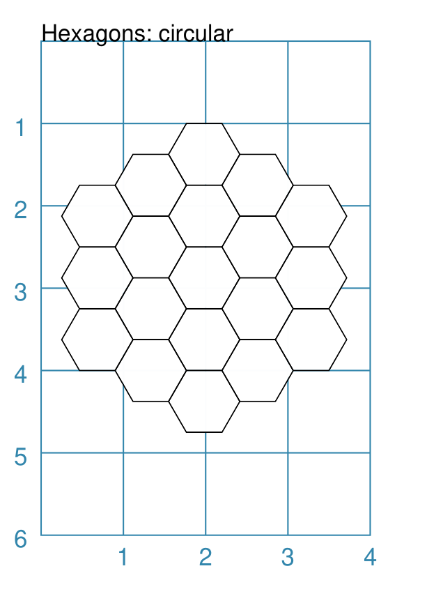
Circular Hexagonal Grid
An alternative to the basic hexagonal grid, is a circular, or circle, layout.
Thes are sometimes termed “hexhex” grids.
Most of the properties that associated with the basic grid are can also be used for the circular grid: coordinates; caltrops; radii and hidden hexagons.
Basic
|
This example shows a grid constructed using the command: Hexagons(
x=0.25, y=1,
height=0.75,
sides=3,
fill="white",
hex_layout="circle",
)
It has the following properties that differ from the defaults:
|
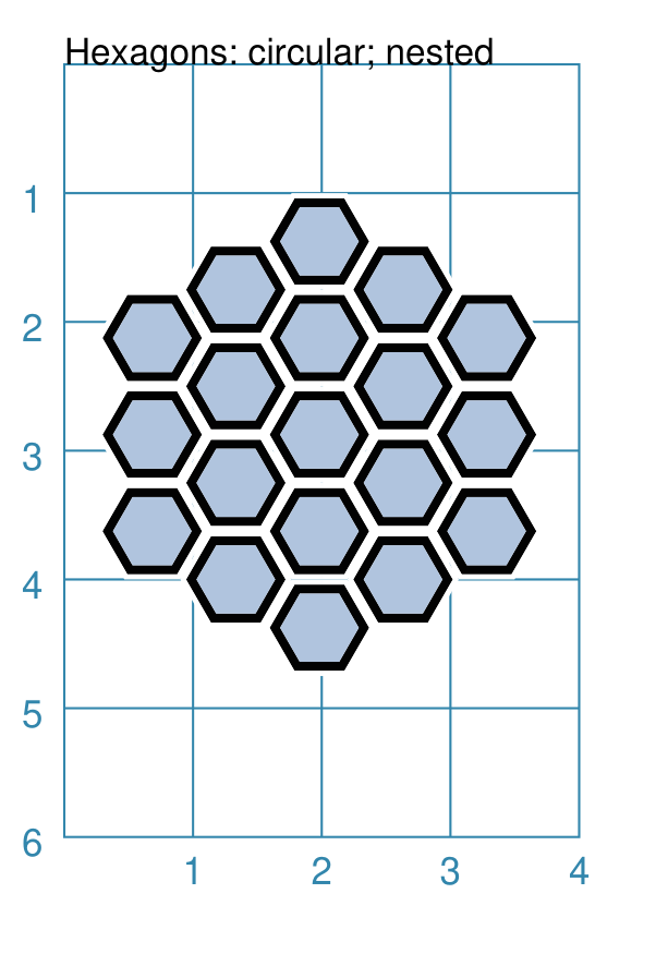
Nested Shapes
|
This example shows a grid constructed using the command: Hexagons(
x=0.25, y=1,
height=0.75,
sides=3,
stroke=None, fill="white",
hex_layout="circle",
centre_shape=hexagon(
stroke="black",
fill="lightsteelblue",
height=0.6, stroke_width=2),
)
It has the following properties that differ from the defaults:
The centre point of the centre_shape aligns with the centre of the hexagon. The location of the centre_shape will match that of the hexagon
within which it is “nested”; in this case its size is smaller
— |
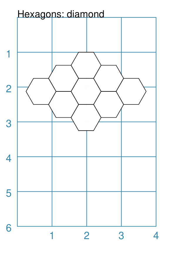
Diamond Hexagonal Grid
An alternative to the basic hexagonal grid, is a diamond layout.
Most of the properties that associated with the basic grid are can also be used for the diamond grid: coordinates; caltrops; radii and hidden hexagons.
Basic
|
This example shows a grid constructed using the command: Hexagons(
x=0.25, y=1,
height=0.75,
rows=3,
fill="white",
hex_layout="diamond",
)
It has the following properties that differ from the defaults:
|
Grid Locations
In order to layout objects within a hexagonal grid, it is possible to use
the Location() or Locations() command to specify the “what, where
and how”.
These commands should work with any of the types of hexagonal grid layouts described above.
The following are the key properties required for the Location() or the
Locations() command:
grid - a grid, or the name assigned to a grid
coordinates - these are coordinates assigned when creating the grid; if none have been assigned, the default numbering is used i.e. a label made up of two 2-digit numbers (each padded with zero) which correspond to the row and column - bear in mind the numbering starts at the top-left of the grid
shapes - a list (using square brackets [ and ]) of one of more shapes, appearing in the order that they must be drawn; the centre of the shapes will be set to match the centre of the hexagon in which its drawn.
All examples below make use of a common property (assigned to the name a_circle) defined as:
a_circle = Common(radius=0.4)
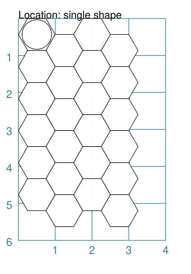
Location
Example 1. Single Shape
|
This example shows a location constructed using the command: hexgrid = Hexagons(
side=0.5,
x=0, y=0,
rows=6, cols=4,
)
Location(
hexgrid,
"0101",
[circle(common=a_circle)]
)
The The grid is assigned the name hexgrid so it’s result can be reused. The
The Location’s list contains just one shape — a |
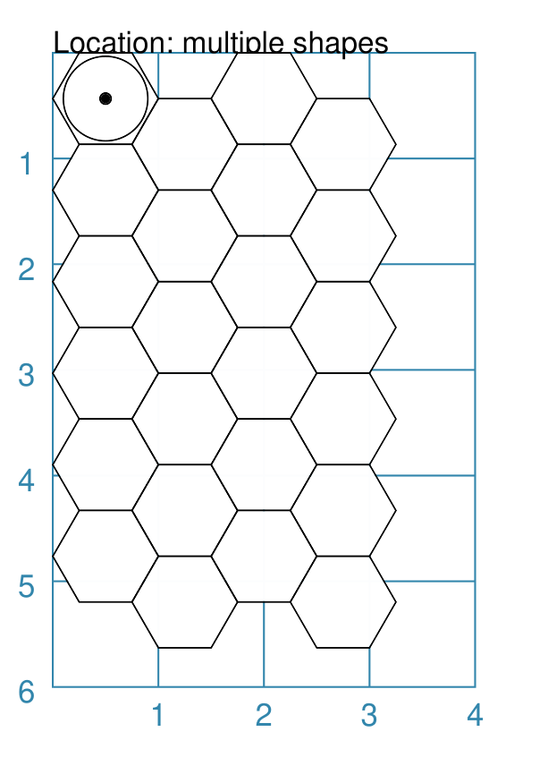
Example 2. Multiple Shapes
|
This example shows a location constructed using the command: hexgrid = Hexagons(
side=0.5,
x=0, y=0,
rows=6, cols=4,
)
Location(
hexgrid,
"0101",
[circle(common=a_circle), dot()]
)
The The grid is assigned the name hexgrid so it’s result can be reused. The
The list contains two shapes — a |
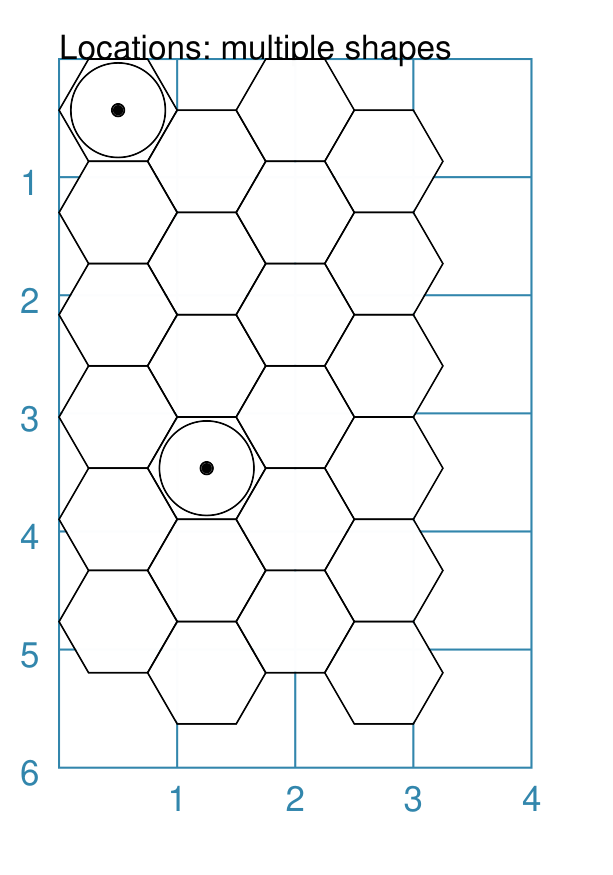
Locations
It is often the case that the same shape, or set of shapes, needs to be displayed at multiple locations within the grid.
Example 1. Locations and Shapes
|
This example shows locations constructed using the command: hexgrid = Hexagons(
side=0.5,
x=0, y=0,
rows=6, cols=4,
)
Locations(
hexgrid,
"0204, 0101",
[circle(common=a_circle), dot()]
)
The The grid is assigned the name hexgrid so it’s result can be reused. The
The list contains two shapes — a |
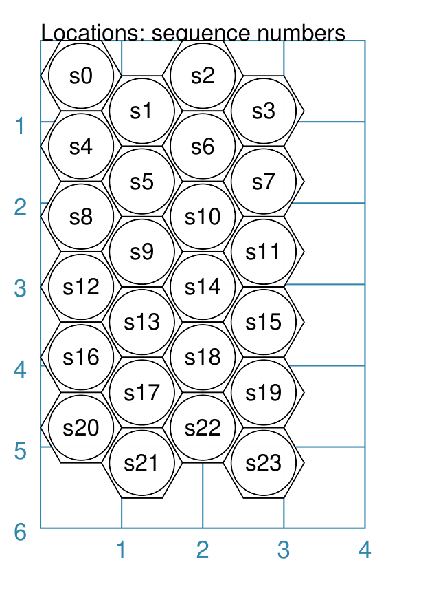
Example 2. Locations & Sequence
|
This example shows locations constructed using the command: hexgrid = Hexagons(
side=0.5,
x=0, y=0,
rows=6, cols=4,
)
Locations(
hexgrid,
"all",
[circle(common=a_circle, label="s{{sequence}}")]
)
The The grid is assigned the name hexgrid so it’s result can be reused. The
The list contains a single shape — a Because of the enclosing brackets |
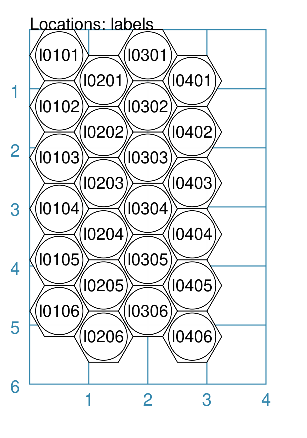
Example 3. Locations & Labels
|
This example shows locations constructed using the command: hexgrid = Hexagons(
side=0.5,
x=0, y=0,
rows=6, cols=4,
)
Locations(
hexgrid,
"all",
[circle(common=a_circle, label="l{{label}}")]
)
The The grid is assigned the name hexgrid so it’s result can be reused. The
The list contains a single shape — a Because of the enclosing brackets |
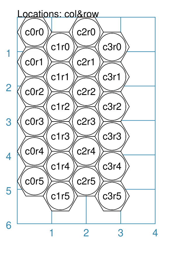
Example 4. Locations & Col/Row
|
This example shows locations constructed using the command: hexgrid = Hexagons(
side=0.5,
x=0, y=0,
rows=6, cols=4,
)
Locations(
hexgrid,
"all",
[circle(
common=a_circle,
label="c{{col}}r{{row}}")]
)
The The grid is assigned the name hexgrid so it’s result can be reused. The
The list contains a single shape — a Because of the enclosing brackets |
Grid GridLine
The GridLine() command allows the creation of a line, or lines, joining,
or running along or between the edges of, one or more hexagons within a
hexagonal grid.
This command should work with any of the types of hexagonal grid layouts described above.
Hint
One example of the use of the GridLine command is drawing features
on a hex-gridded map; such as tracks, roads, railways / railroads,
rivers, hedges, regional boundaries or borders, or any other similar
linear features.
See an example wargame board for
such applications of the GridLine command.
GridLine Properties
The GridLine() command has the following key properties:
hexgrid - this is the first property that must be assigned; it is the name of a
Hexagons()grid that must already have been created by the scriptlocations - a set of locations in the grid; either as a string containing comma-separated values or as a list (using square brackets [ and ]`); these location’s centres will be joined by straight lines
edges - a set of directions in the grid; either as a string containing comma-separated values or as a list (using square brackets [ and ]`); these will result in a continous line along hexagon edges
paths - a set of directions in the grid; either as a string containing comma-separated values or as a list (using square brackets [ and ]`); these will result in a continous line between hexagon edges
For the edges and paths to work, the following properties must also be set:
start - this is a named location in the grid
point - this a compass-based point reference for the starting hexagon — either a vertex for paths; or a perbis (centre point of an edge) for edges
The GridLine can be styled by setting the usual styling properties that
are applicable to a Line.
GridLine Examples
All of the examples below make use of the same underlying hexagonal grid:
hexgrid = Hexagons(
    side=0.5,
    x=0, y=0,
    rows=6, cols=4,
    dot=0.02,
    coord_elevation='top'
)
This grid is assigned the name hexgrid so its result can be reused.
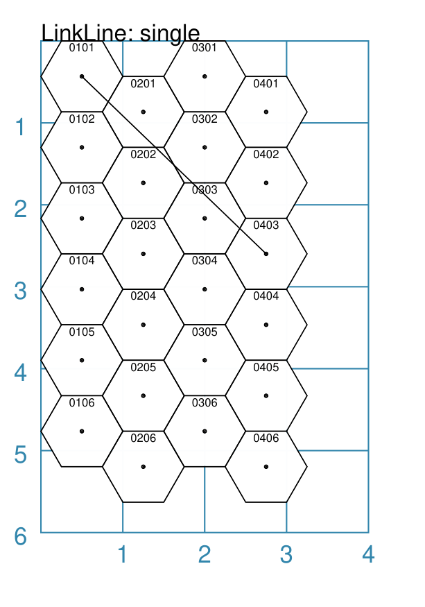
Example 1. A Single GridLine
|
This example shows a GridLine(
grid=hexgrid,
locations="0101,0403"
)
The
The locations represent the coordinates of the start and end locations in the grid, between which the line is drawn. By default, the |
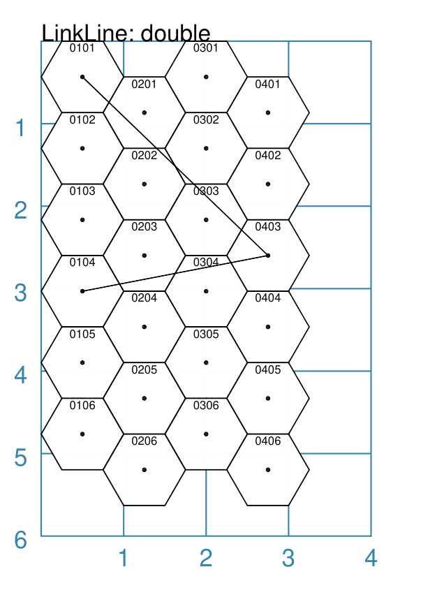
Example 2. A Double GridLine
|
This example shows a GridLine(
hexgrid,
locations="0101,0403,0104"
)
The
The string contains the coordinates of multiple start and end locations in the grid, between which the line is drawn. The first lines is drawn between the first and second hexagon; the second between the second and third hexagon specified. By default, the Note that in this example, the |
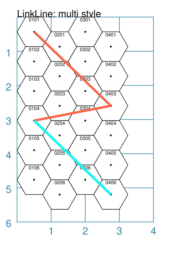
Example 3. A Styled GridLine
|
This example shows a GridLine(
hexgrid,
locations=["0101", "0403", "0104", "0406"],
common=Common(
stroke="tomato",
stroke_width=2)
)
GridLine(
hexgrid,
locations=["0104", "0406"],
common=Common(
stroke="cyan",
stroke_width=2)
)
The
The location coordinates contain multiple start and end locations in the grid, between which the lines are drawn. In this example, the locations are defined as individual strings in a list. By default, the lines use the x and y values of the centre of the hexagon in which they start or end. |
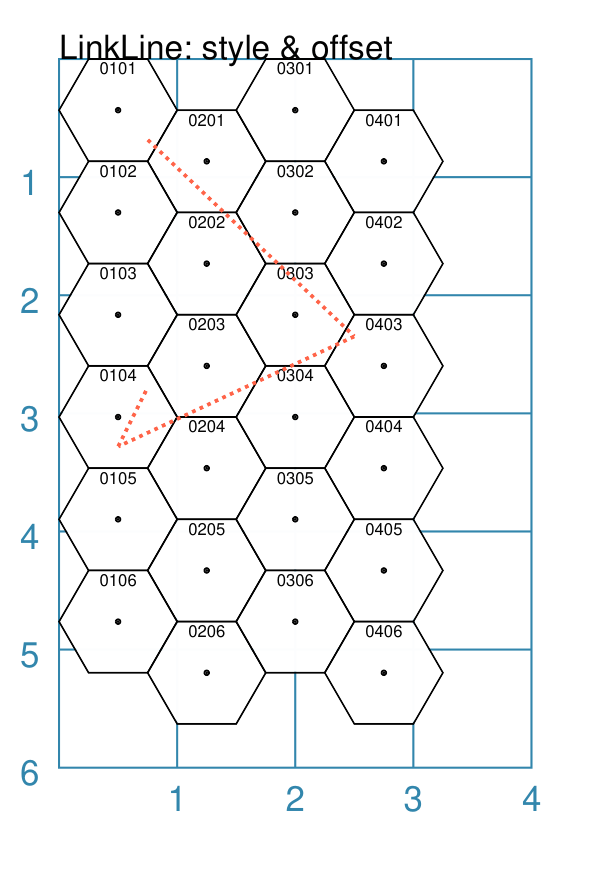
Example 4. An Offset GridLine
|
This example shows a GridLine(
hexgrid,
locations=[
("0101", 0.25, 0.25),
("0403", -0.25, -0.25),
("0104", 0.0, 0.25),
("0104", 0.25, -0.25)],
common=Common(
stroke="tomato",
stroke_width=1,
dotted=True)
)
The
The offset values — x and y — are distances that are relative to the centre of the hexagon in which the line starts or ends. Positive values for the offset move the x and y down and to the right of the centre; negatives move the x and y up and to the left of the centre. Note that its possible to define the start and end as different offsets
within the same hexagon; as shown here for location |
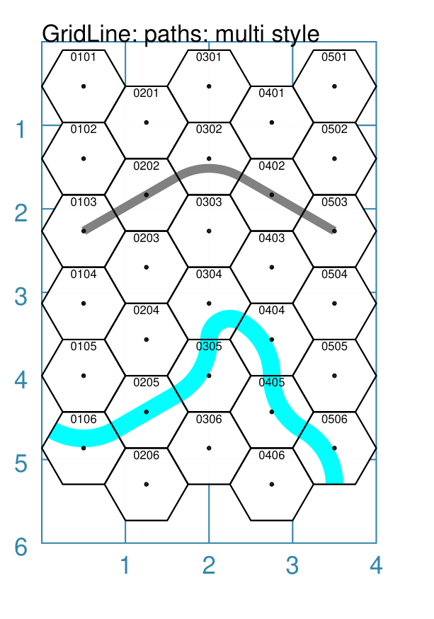
Example 5. GridLine as a Path
|
This example shows the use of the hexgrid = Hexagons(
side=0.5,
x=0, y=0.1,
rows=6, cols=5,
)
GridLine(
hexgrid,
start="0106",
point="nw",
paths=["ne", "ne", "n", "se", "s", "se", "s"],
stroke="cyan",
stroke_width=6
)
GridLine(
hexgrid,
start="0103",
point="c",
paths="ne,ne,se,se,c",
stroke="grey",
stroke_width=3
)
Hexagons(
side=0.5,
x=0, y=0.1,
rows=6, cols=5,
dot=0.02,
coord_elevation='top',
fill=None
)
The
The paths can be specified either as:
|
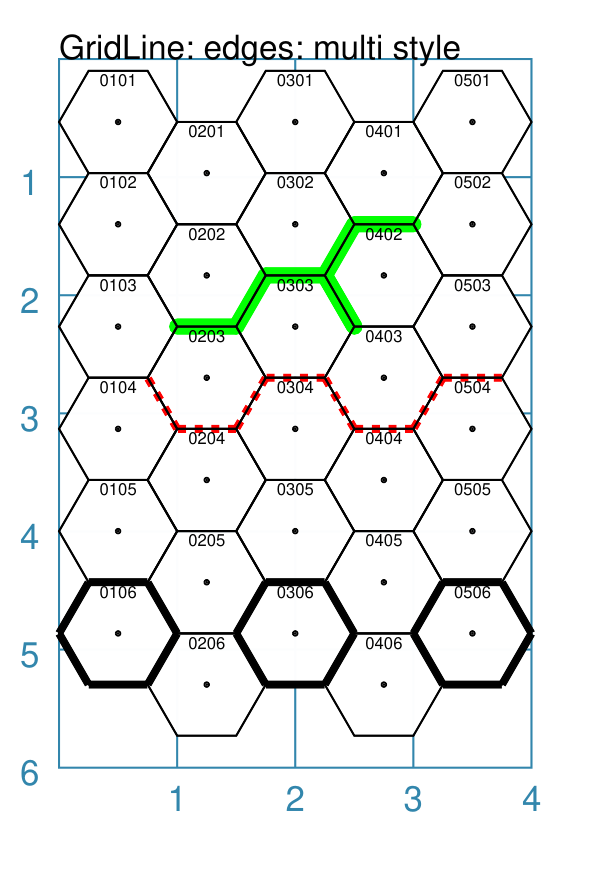
Example 6. GridLine along Edges
|
This example shows the use of the hexgrid = Hexagons(
side=0.5, x=0, y=0.1, rows=6, cols=5)
GridLine(
hexgrid,
start="0203",
point="nw",
edges="e,ne,e,se,nw,ne,e",
stroke="green",
stroke_width=4,
stroke_ends="rounded"
)
GridLine(
hexgrid,
start="0504",
point="ne",
edges=["w", "sw", "w", "nw"] * 2,
stroke="red",
stroke_width=2,
dotted=True
)
GridLine(
hexgrid,
start=["0106", "0306", "0506"],
point="ne",
edges="*",
stroke="black",
stroke_width=2
)
Hexagons(
side=0.5,
x=0, y=0.1,
rows=6, cols=5,
fill=None,
dot=0.02,
coord_elevation='top'
)
A
The edges can be specified either as:
Note the the various line styling properties affect how the line is drawn — as oppposed to where it is drawn. |
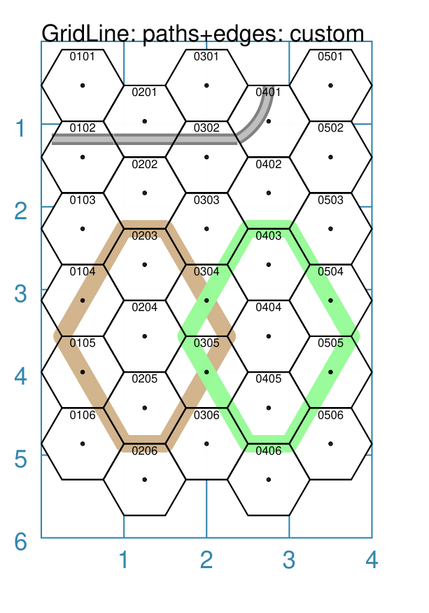
Example 7. GridLine Custom Paths and Edges
|
This example shows the use of the hexgrid = Hexagons(
side=0.5,
x=0, y=0.1,
rows=6, cols=5,
)
road = "ne=,se=,ne=,n"
GridLine(
hexgrid,
start="0102",
point="nw",
paths=road,
stroke="grey",
stroke_width=4
)
GridLine(
hexgrid,
start="0102",
point="nw",
paths=road,
stroke="silver",
stroke_width=2
)
GridLine(
hexgrid,
start="0104",
point="sw",
edges="ne,ne,e,se,se,sw,sw,w,nw,nw",
stroke="tan",
stroke_width=6,
stroke_ends="rounded"
)
GridLine(
hexgrid,
start="0504",
point="se",
edges="nw,nw,w,sw,sw,se,se,e,ne,ne",
stroke="palegreen",
stroke_width=6,
stroke_ends="rounded"
)
Hexagons(
side=0.5,
x=0, y=0.1,
rows=6, cols=5,
dot=0.02,
coord_elevation='top',
fill=None
)
As in other examples,
In the upper example, the paths property is assigned to a name —
road — which has been defined as a series of directions; some
of which have an equal sign In addition, the upper example shows how two lines can be drawn on the same path to create a styled effect: in this case, the thinner, light grey line is drawn over the thicker, dark grey line. In the lower two examples, the edges property is used to draw lines from the corner (or vertex) of a hexagon to the opposite corner (or vertex). No special symbols are are required for this. Note that while the two outcomes — brown and green lines — look the same, that one is drawn in a clockwise direction and the other in an anti-clockwise direction. |
Other Hexagonal Grid Resources
There are already a number of software tools available for creating hexagonal grids of various kinds and for different purposes.
A few of these tools, some of which are game-specific, for example, the so-called 18XX series, are listed below:
HEXGRID (https://hamhambone.github.io/hexgrid/) - an online hex grid generator which interactively creates a display, downloadable as a PNG image.
mkhexgrid (https://www.nomic.net/~uckelman/mkhexgrid/) - a command-line program which generates hexagonal grids, used for strategy games, as PNG or SVG images.
Hex Map Extension (https://github.com/lifelike/hexmapextension/tree/master) - an extension for creating hex grids in Inkscape that can also be used to make brick patterns of staggered rectangles.
hexboard (https://www.ctan.org/pkg/hexboard) - a package for LATEX that provides functionality for drawing boards and game pieces for the abstract game “Hex”
draw_game_board (https://github.com/jpneto/draw_game_boards/tree/main) - a Python tool to translate boards from ASCII format into SVG.
map18xx (https://github.com/XeryusTC/map18xx) - a 18XX hex map and tile generator that outputs to SVG files, scaled to fit A4 paper.
18xx Maker (https://www.18xx-maker.com/) - uses 18XX game definitions written in JSON, displays them, and renders them for printing.
ps18xx (https://github.com/18xx/ps18xx/tree/master) - software for running 18XX email games, and creating maps and tile sheets.
LATEX wargame package (https://wargames_tex.gitlab.io/wargame_www/tools.html) - a package for LaTeX for authoring hex’n’counter wargames.
The options and facilities provided by these tools have been the primary inspiration for how hexagonal grids work in protograf. If the functionality available here does not work for you, then possibly one of these other tools might be a better fit.
Hint
For everything — and I mean everything — related to how hexagonal grids are designed and calculated, the single most useful reference for a designer is https://www.redblobgames.com/grids/hexagons/
An 18XX Footnote
The 18XX game series hex maps are often criticised for their poor aesthetic. A fascinating article that deals with this topic - and is perhaps relevant even at the prototyping stage being supported by this program - can be found at https://medium.com/grandtrunkgames/mawgd4-18xx-tiles-and-18xx-maps-8a409bba4230