Shapes Geometry

The descriptions here assume you are familiar with the concepts, terms and ideas for protograf as presented in the Basic Concepts — especially units, properties and defaults.

You should have already seen how these shapes were created, with defaults, in Core Shapes. You will also need to understand how shapes can be further customised

Overview
Point-based Locations
Geometry Properties
Examples of using Named Geometry Properties

Overview

↑

When reading this section, you should already know how shapes are created by using commands, and understand how their properties are set.

This section describes the use of point locations to set where shapes are drawn. It also covers the availability and use of a shape’s geometry properties that can be used to set relative locations e.g. given that a Rectangle has been drawn, use a relative reference to its north-east corner.

Point-based Locations

↑

For the majority of shapes, their location is typically set either by supplying their x and y values to define the top-left position of the shape — with both values defaulting to 1 — or through using their cx and cy values to define the centre position of the shape — with both values defaulting to 1.

It is also possible to use the xy property or cxy property to achieve the same result; the difference being that the script needs to provide values for these properties using a Point command rather than a single number.

The Point() command simply uses two values — if not names are used, then it us s assumed that these correspond to the x and y properties; in that order.

For example, in all cases below the top-left of the Rectangle is at x-position 2 and y-position 3:

Rectangle(x=2, y=3)
Rectangle(xy=Point(x=2, y=3))
Rectangle(xy=Point(2, 3))

In this example, in all cases below the centre of the Rectangle is at x-position 1 and y-position 4:

Rectangle(cx=1, cy=4)
Rectangle(cxy=Point(x=1, y=4))
Rectangle(cxy=Point(1, 4))

Setting locations this way is more verbose and perhaps less immediately clear than using single properties. However, it might be of use in some cases — and is certainly needed when referencing another shape’s geometry (see below).

Geometry Properties

↑

Much of protograf’s documentation and focus is on setting of properties for shapes so that they appear the way you want them to. However, it can be useful to reuse those properties to allow for more flexibility and ease-of-change in a script.

Using a Property

Each shape, depending on its characteristics, has various geometry properties available.

Warning

The correct geometry properties only become available after a shape has been drawn!

Geometry properties are referenced using a NAME.geo.XYZ syntax; where the NAME is a name assigned in the script to the shape, and the XYZ is the property being referenced. For example:

box = Rectangle(cx=1, cy=4, height=2, width=5)
Circle(cxy=box.geo.c, radius=1)

Here the name box is assigned to the Rectangle, and the Circle’s centre point is set by referencing the Rectangle’s centre point via the box.geo.c, where the c refers to the centre.

Hint

You can also refer to a shape’s geometry properties by using the terms in full — for example, box.geometry.centre

A Circle also has clock locations available; see - Example 5. Circle Named and Other Points.

Available Properties

There are a number of potentially available properties. Obviously, though, their value may or may not exist depending on the shape involved. For example, circular-like shapes such as a Circle, Hexagon and Polygon have a radius, whereas shapes such as a Rhombus, Rectangle or Cross do not.

Named Location Properties

Locations refer to key points for a shape.

Key points include: the shape centre — common to most shapes; the vertices which help define its “outer” lines; and, for specific shapes, the perbii i.e. the mid-points of the lines between two vertices at which the lines from the centre of the shape form right-angles to them.

Locations are typically referenced via compass directions which match the location, relative to the shape’s centre, in an exact or approximate way. These include:

n - a point on the north edge or vertex
s - a point on the south edge or vertex
e - a point on the east edge or vertex
w - a point on the west edge or vertex
ne - a point on the north-east edge or vertex
se - a point on the south-east edge or vertex
nw - a point on the north-west edge or vertex
sw - a point on the south-west edge or vertex
nnw - a point on the north-north-west edge or vertex
nne - a point on the north-north-east edge or vertex
sse - a point on the south-south-east edge or vertex
ssw - a point on the south-south-west edge or vertex
wnw - a point on the west-north-west edge or vertex
ene - a point on the east-north-east edge or vertex
ese - a point on the east-south-east edge or vertex
wsw - a point on the west-south-west edge or vertex

Usage of these is shown in Example 4. Hexagonal Vertices and Perbii as well as Example 5. Circle Named and Other Points.

Numbered Location Properties

It is not always possible access locations by name. For some shapes, such as a Polygon or Star, they can only be referenced by a number.

Numbered locations include:

vertices (v) — a list of vertices for the shape, where each item is referenced by a number, starting from 0.
perbii (p) — a list of perbii for the shape, where each item is referenced by a number, starting from 0.

As an example:

ply = Polygon(cx=1, cy=4, sides=7, side=1)
Line(xy=ply.geo.v[3], length=1)

Here the Line uses, as its starting point, the fourth vertex of the 7-sided Polygon named ply.

See Example 3. Use of Vertices for Polygon for use of numbered locations.

Size Properties

In general, size properties are associated with regular, enclosed shapes.

area - the area of the shape
perimeter - the length of the line around the shape
radius - the radius of the shape, where applicable
diameter - the diameter of the shape, where applicable
side - the length of a side of the shape (if all sides are equal)
length - the length of the shape (if it has a single length)
width - the width of the shape (if it has a single width)
height - the height of the shape (if it has a single height)
sides - the number of sides of the shape (if all sides are of equal length)

Warning

Be aware that calculations are not yet in place for some, or all, of these calculated values, or that the calculations themselves may still only be approximations — use these properties with caution for now!

Non-Numeric Properties

type - the shape type (the internal protograf type)
name - the shape’s name is usually the same as its command (this property does not refer to any name that might have been assigned to it in a script)

Examples of using Named Geometry Properties

↑

Example 1. Named Properties
Example 2. Use of Named Points for Shapes
Example 3. Use of Vertices for Polygon
Example 4. Hexagonal Vertices and Perbii
Example 5. Circle Named and Other Points

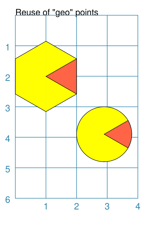
Example 1. Named Properties

^

This example shows named points referenced using these commands:

hx = Hexagon(
  x=0, y=0.85, height=2,
  fill="yellow",
  orientation="pointy")
Polyshape(
  points=[hx.geo.c, hx.geo.ne, hx.geo.se],
  fill="tomato")

cc = Circle(
  x=2, y=3, radius=0.9,
  fill="yellow")
Sector(
  cxy=cc.geo.c,
  radius=cc.geo.radius,
  angle_width=60,
  angle_start=-30,
  fill="tomato")

The two “primary” shapes — Hexagon and Circle — are assigned names (hx and cc respectively).

These are then used to gain access to their geometric properties.

For example, the triangular Polyshape is drawn over the Hexagon by referencing various of its available vertices for use in the points property.

The Sector is drawn over the Circle by referencing both the radius and the centre of the Circle (assigned to cxy).

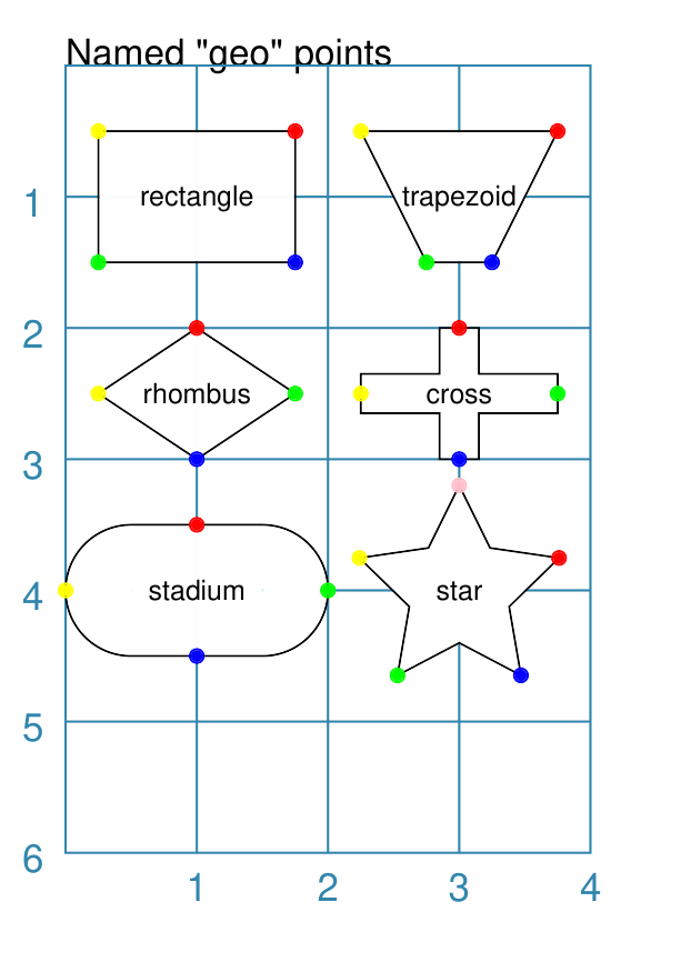
Example 2. Use of Named Points for Shapes

^

This example shows named points referenced using these commands:

sh = Rectangle(
    cx=1, cy=1, height=1, width=1.5,
    label="rectangle", label_size=6)
Dot(cxy=sh.geo.ne, fill_stroke="red")
Dot(cxy=sh.geo.se, fill_stroke="blue")
Dot(cxy=sh.geo.sw, fill_stroke="green")
Dot(cxy=sh.geo.nw, fill_stroke="yellow")
sh = Trapezoid(
    cx=3, cy=1, height=1, width=1.5,
    label="trapezoid", label_size=6)
Dot(cxy=sh.geo.ne, fill_stroke="red")
Dot(cxy=sh.geo.se, fill_stroke="blue")
Dot(cxy=sh.geo.sw, fill_stroke="green")
Dot(cxy=sh.geo.nw, fill_stroke="yellow")
sh = Rhombus(
    cx=1, cy=2.5, height=1, width=1.5,
    label="rhombus", label_size=6)
Dot(cxy=sh.geo.n, fill_stroke="red")
Dot(cxy=sh.geo.s, fill_stroke="blue")
Dot(cxy=sh.geo.e, fill_stroke="green")
Dot(cxy=sh.geo.w, fill_stroke="yellow")
sh = Cross(
    cx=3, cy=2.5, height=1, width=1.5,
    label="cross", label_size=6)
Dot(cxy=sh.geo.n, fill_stroke="red")
Dot(cxy=sh.geo.s, fill_stroke="blue")
Dot(cxy=sh.geo.e, fill_stroke="green")
Dot(cxy=sh.geo.w, fill_stroke="yellow")
sh = Stadium(
    cx=1, cy=4, height=1, width=1,
    label="stadium", label_size=6)
Dot(cxy=sh.geo.n, fill_stroke="red")
Dot(cxy=sh.geo.s, fill_stroke="blue")
Dot(cxy=sh.geo.e, fill_stroke="green")
Dot(cxy=sh.geo.w, fill_stroke="yellow")
sh = Star(
    cx=3, cy=4, radius=0.8, rays=5,
    label="star", label_size=6)
Dot(cxy=sh.geo.v[0], fill_stroke="red")
Dot(cxy=sh.geo.v[1], fill_stroke="blue")
Dot(cxy=sh.geo.v[2], fill_stroke="green")
Dot(cxy=sh.geo.v[3], fill_stroke="yellow")
Dot(cxy=sh.geo.v[4], fill_stroke="pink")

This example shows the “equivalence” between use of compass directions for a number of different shapes.

Note that the Stadium points will lie on a curve if it has edges that “bulge” in that direction;

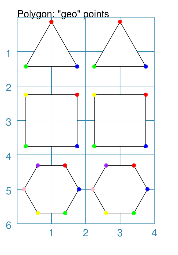
Example 3. Use of Vertices for Polygon

^

This example shows numbered and named points referenced using these commands:

p1 = Polygon(x=1, y=1, sides=3, side=1.5)
Dot(cxy=p1.geo.n, fill_stroke="red")
Dot(cxy=p1.geo.se, fill_stroke="blue")
Dot(cxy=p1.geo.sw, fill_stroke="green")
p2 = Polygon(x=3, y=1, sides=3, side=1.5)
Dot(cxy=p2.geo.v[2], fill_stroke="red")
Dot(cxy=p2.geo.v[0], fill_stroke="blue")
Dot(cxy=p2.geo.v[1], fill_stroke="green")

p1 = Polygon(x=1, y=3, sides=4, side=1.5)
Dot(cxy=p1.geo.ne, fill_stroke="red")
Dot(cxy=p1.geo.se, fill_stroke="blue")
Dot(cxy=p1.geo.sw, fill_stroke="green")
Dot(cxy=p1.geo.nw, fill_stroke="yellow")
p2 = Polygon(x=3, y=3, sides=4, side=1.5)
Dot(cxy=p2.geo.v[0], fill_stroke="red")
Dot(cxy=p2.geo.v[1], fill_stroke="blue")
Dot(cxy=p2.geo.v[2], fill_stroke="green")
Dot(cxy=p2.geo.v[3], fill_stroke="yellow")

p1 = Polygon(x=1, y=5, sides=6, side=0.8)
Dot(cxy=p1.geo.ne, fill_stroke="red")
Dot(cxy=p1.geo.e, fill_stroke="blue")
Dot(cxy=p1.geo.se, fill_stroke="green")
Dot(cxy=p1.geo.sw, fill_stroke="yellow")
Dot(cxy=p1.geo.w, fill_stroke="pink")
Dot(cxy=p1.geo.nw, fill_stroke="purple")
p2 = Polygon(x=3, y=5, sides=6, side=0.8)
Dot(cxy=p2.geo.v[0], fill_stroke="red")
Dot(cxy=p2.geo.v[1], fill_stroke="blue")
Dot(cxy=p2.geo.v[2], fill_stroke="green")
Dot(cxy=p2.geo.v[3], fill_stroke="yellow")
Dot(cxy=p2.geo.v[4], fill_stroke="pink")
Dot(cxy=p2.geo.v[5], fill_stroke="purple")

This example shows the “equivalence” between use of compass directions versus numbered vertices (such as v[0]). The named directions can only be used for these polygons because of their smaller number of sides.

Other sizes of polygons will not have any named locations available, and to reference their vertices will require the use of numbers.

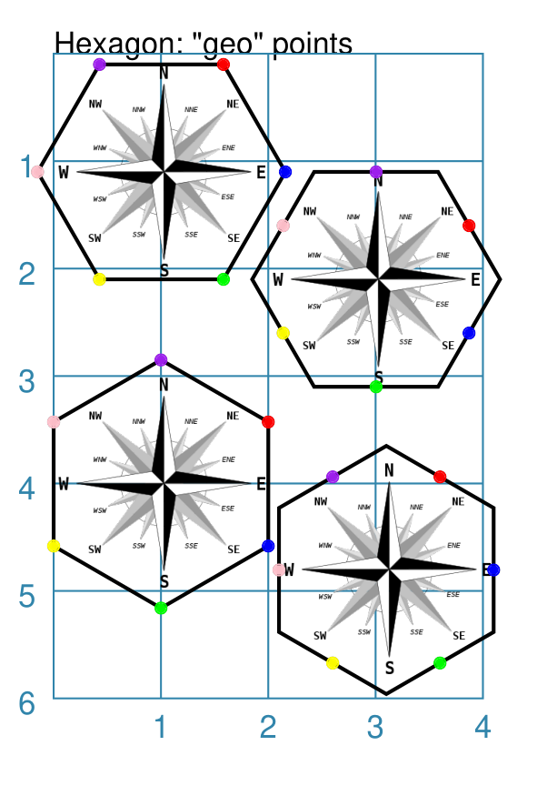
Example 4. Hexagonal Vertices and Perbii

^

This example shows the points that can be referenced using these commands:

Image(
  "compass.png",
  x=0, y=0.1, height=2, width=2)
hx = Hexagon(
  x=-0.15, y=0.1, height=2,
  fill=None, stroke_width=1)
Dot(cxy=hx.geo.ne, fill_stroke="red")
Dot(cxy=hx.geo.e, fill_stroke="blue")
Dot(cxy=hx.geo.se, fill_stroke="green")
Dot(cxy=hx.geo.sw, fill_stroke="yellow")
Dot(cxy=hx.geo.w, fill_stroke="pink")
Dot(cxy=hx.geo.nw, fill_stroke="purple")

Image(
  "compass.png",
  x=2, y=1.1, height=2, width=2)
hx = Hexagon(
  x=1.85, y=1.1, height=2,
  fill=None, stroke_width=1)
Dot(cxy=hx.geo.ene, fill_stroke="red")
Dot(cxy=hx.geo.ese, fill_stroke="blue")
Dot(cxy=hx.geo.s, fill_stroke="green")
Dot(cxy=hx.geo.wsw, fill_stroke="yellow")
Dot(cxy=hx.geo.wnw, fill_stroke="pink")
Dot(cxy=hx.geo.n, fill_stroke="purple")

Image(
  "compass.png",
  x=0, y=3, height=2, width=2)
hx = Hexagon(
  x=0, y=2.85, height=2, fill=None,
  stroke_width=1, orientation="pointy")
Dot(cxy=hx.geo.ne, fill_stroke="red")
Dot(cxy=hx.geo.se, fill_stroke="blue")
Dot(cxy=hx.geo.s, fill_stroke="green")
Dot(cxy=hx.geo.sw, fill_stroke="yellow")
Dot(cxy=hx.geo.nw, fill_stroke="pink")
Dot(cxy=hx.geo.n, fill_stroke="purple")

Image(
  "compass.png",
  x=2.1, y=3.8, height=2, width=2)
hx = Hexagon(
  x=2.1, y=3.65, height=2, fill=None,
  stroke_width=1, orientation="pointy")
Dot(cxy=hx.geo.nne, fill_stroke="red")
Dot(cxy=hx.geo.e, fill_stroke="blue")
Dot(cxy=hx.geo.sse, fill_stroke="green")
Dot(cxy=hx.geo.ssw, fill_stroke="yellow")
Dot(cxy=hx.geo.w, fill_stroke="pink")
Dot(cxy=hx.geo.nnw, fill_stroke="purple")

These four Hexagons each show a different aspect of using named locations. In all cases, a series of colored Dots are drawn, in the same sequence, in a clockwise direction.

While vertices can be easily identified with primary or secondary compass directions, some of the perbii can only be identified by tertiary compass directions.

The compass image provides some context to see how the named locations are only approximations to the actual compass directions.

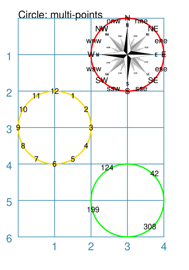
Example 5. Circle Named and Other Points

^

A Circle has three different ways to locate a point on its circumference.

This example shows the points that can be referenced using these commands:

cr = Circle(cx=3, cy=1, radius=1, fill=None, stroke_width=1, stroke="red")
dcp = Common(dot_width=2, stroke="red", label_stroke="black")
Dot(common=dcp, label="N", cxy=cr.geo.n)
Dot(common=dcp, label="S", cxy=cr.geo.s)
Dot(common=dcp, label="E", cxy=cr.geo.e)
Dot(common=dcp, label="W", cxy=cr.geo.w)
...
cr = Circle(cx=1, cy=3, radius=1, fill=None, stroke_width=1, stroke="gold")
dcc = Common(dot_width=2, stroke="gold", label_stroke="black")
Dot(common=dcc, label="12", cxy=cr.clock.h12)
Dot(common=dcc, label="9", cxy=cr.clock.h9)
Dot(common=dcc, label="6", cxy=cr.clock.h6)
Dot(common=dcc, label="3", cxy=cr.clock.h3)
...
cr = Circle(cx=3, cy=5, radius=1, fill=None, stroke_width=1, stroke="green")
Text("42", xy=cr.poc(42))
Text("124", xy=cr.poc(124))
Text("308", xy=cr.poc(308))
Text("199", xy=cr.poc(199))

NOTE that the code shown above is abbreviated (...) but the pattern of usage should be clear from what is here.

The red circle shows the use of named compass points; all sixteen are available for a circle.

The yellow circle shows the use of named clock points; these are referenced using a NAME.clock.hN syntax; where NAME is the name assigned in the script to the Circle, and the hN is an h followed by a number corresponding to an hour position.

The green circle shows the use of angles to set a location. The format is NAME.poc(N) where NAME is the name assigned in the script to the Circle, and the poc(N) is the method by which an angle in degrees, between 0 to 360, measured counter-clockwise from the east direction, can be specified.