DiamondLocations Command
This section assumes you are very familiar with the concepts, terms and ideas for protograf as presented in the Basic Concepts , that you understand all of the Additional Concepts and that you’ve created some basic scripts of your own using the Core Shapes.
This is part of the set of commands used for Layouts, that are used in conjunction with the Layout command.
Overview
The DiamondLocations() command defines an ordered series
of row and column locations that create a diamond pattern i.e
two equilateral triangles placed edge-to-edge. This pattern is
termed a grid.
The x- and y-values of these rows and columns are then used to set the centres of the elements that can be placed there using the Layout() command.
Apart from the DiamondLocations() command described here,
there are also these other commands which allow you to layout
elements in a more repetitive or regular way within a page:
Usage
The DiamondLocations() command accepts the following properties:
x - the horizontal position of the starting point of the grid; this defaults to
1y - the vertical position of the starting point of the grid; this defaults to
1cols - this is the number of locations in the horizontal direction; this defaults to
3(the minimum)rows - this is the number of locations in the vertical direction; this defaults to
3(the minimum)facing - this is the compass point from where the grid is initially drawn; values can be north, south, east and west — this is the default i.e. the left “corner” point
Note
Bear in mind that the DiamondLocations() command is designed
to work in conjunction with a Layout() command
which accepts, as its first property, the name assigned to the grid.
Properties
Many examples below make use of some named Circle shapes which
are defined as:
circles = Common(
    diameter=1.0,
    label="{{sequence}}//{{col}}-{{row}}",
    label_size=6)
a_circle = circle(common=circles)
d_circle = circle(x=0, y=0, radius=0.33)
In these examples, the placeholder names {{sequence}}, {{col}}
and {{row}} will be replaced, in the label for the Circle, by the
values for the row and column in which that circle is placed, as well as
by the sequence number (order) in which that Circle is drawn.
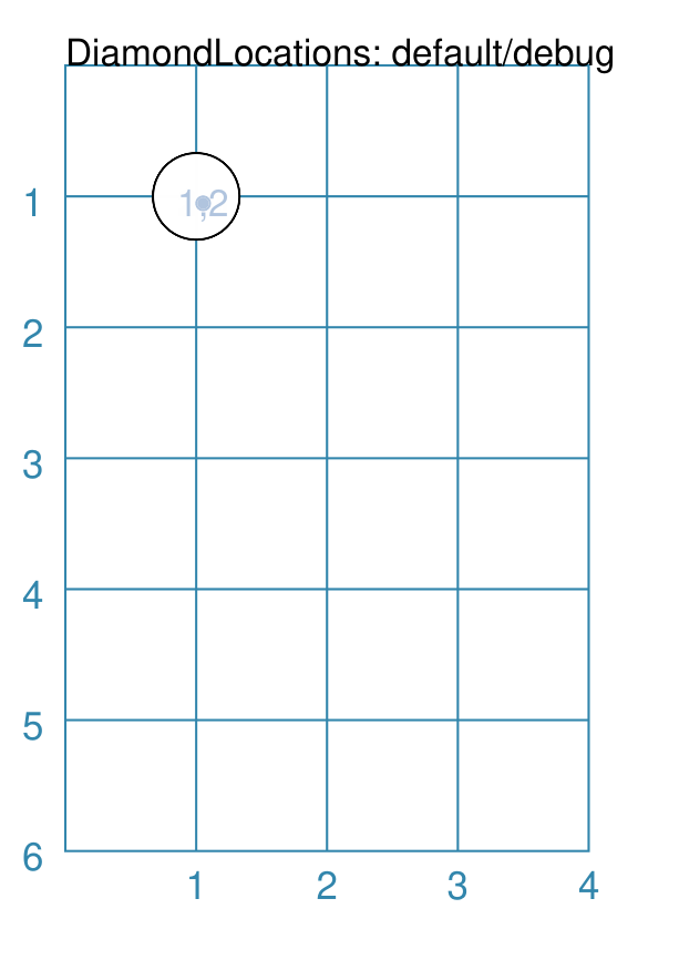
Example 1. Rows and Columns
|
This example shows the shape constructed using differing values for its properties. dia = DiamondLocations()
Layout(
dia, shapes=[d_circle,], debug='cr')
Here, because there is only the default |
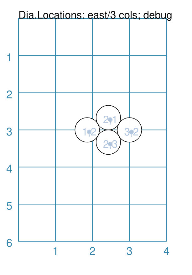
Example 2. East - 3 Columns
|
This example shows the shape constructed using differing values for its properties. dia = DiamondLocations(
facing='east', cols=3,
x=3, y=3, side=0.66)
Layout(
dia, shapes=[d_circle,], debug='cr')
Here, the layout starts on the mid-right side - because the facing
is The debug value shows the column and row values (in that order). |
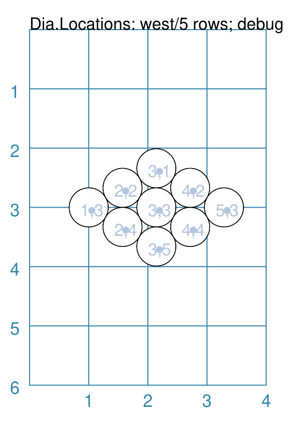
Example 3. West - 5 Rows
|
This example shows the shape constructed using differing values for its properties. dia = DiamondLocations(
facing='west', rows=5,
x=1, y=3, side=0.66)
Layout(
dia, shapes=[d_circle,], debug='cr')
Here, the layout starts on the mid-left side - because the facing
is The debug value shows the column and row values (in that order). |
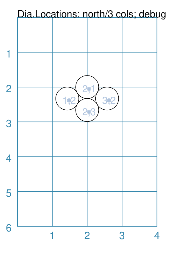
Example 4. North - 3 Columns
|
This example shows the shape constructed using differing values for its properties. dia = DiamondLocations(
facing='north', cols=2,
y=2, x=2, side=0.66)
Layout(
dia, shapes=[d_circle,], debug='cr')
Here, the layout starts on the top-centre side - because the facing
is The debug value shows the column and row values (in that order). |
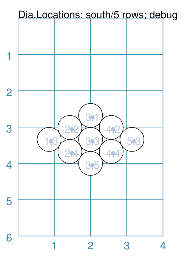
Example 5. South - 5 Rows
|
This example shows the shape constructed using differing values for its properties. dia = DiamondLocations(
facing='south', rows=5,
y=4, x=2, side=0.66)
Layout(
dia, shapes=[d_circle,], debug='cr')
Here, the layout starts on the lower-centre side - because the facing
is The debug value shows the column and row values (in that order). |
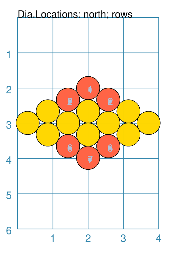
Example 6. Shapes - by Rows
|
This example shows the shape constructed using differing values for its properties. dia = DiamondLocations(
facing='north',
y=2, x=2,
side=.66, cols=7)
Layout(
dia,
shapes=[gold_circle])
Layout(
dia,
shapes=[red_circle],
rows=[1,2,6,7],
debug='r')
Here, two sets of circles are drawn onto the diamond grid. The first set — the The second set — the The debug value in the red circles shows the row number (in order). |
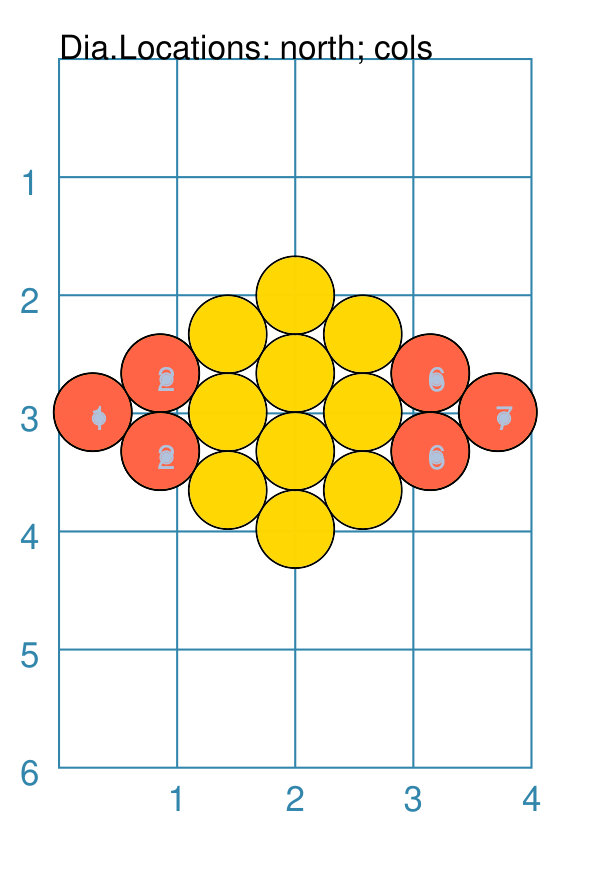
Example 7. Shapes - by Columns
|
This example shows the shape constructed using differing values for its properties. dia = DiamondLocations(
facing='north',
y=2, x=2,
side=.66, cols=7)
Layout(
dia,
shapes=[gold_circle])
Layout(
dia,
shapes=[red_circle],
cols=[1,2,6,7],
debug='c')
Here, two sets of circles are drawn onto the diamond grid. The first set — the The second set — the The debug value in the red circles shows the column number (in order). |
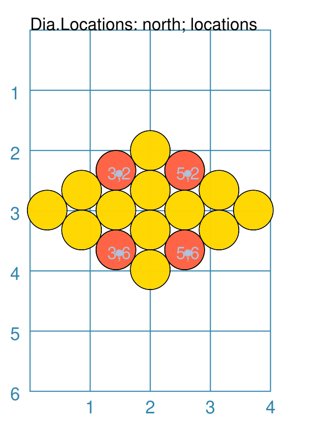
Example 8. Shapes - by Locations
|
This example shows the shape constructed using differing values for its properties. dia = DiamondLocations(
facing='north',
y=2, x=2,
side=.66, cols=7)
Layout(
dia,
shapes=[gold_circle])
Layout(
dia,
shapes=[red_circle],
locations=[
(3,2), (5,2), (3,6), (5,6)],
debug='c')
Here, two sets of circles are drawn onto the diamond grid. The first set — the The second set — the The debug value shows the column and row values (in that order). |
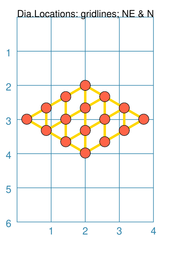
Example 9. Gridlines - Direction
|
This example shows the shape constructed using differing values for its properties. small_circle = circle(
radius=0.15,
fill="tomato")
dia = DiamondLocations(
facing='north',
y=2, x=2,
side=.66, cols=7)
Layout(
dia,
gridlines='ne n',
gridlines_stroke="gold",
gridlines_stroke_width=2,
shapes=[small_circle])
Here, the grid itself is displayed — it is always drawn first before any shapes. The outline of the grid is always drawn. The key prefix is gridlines and the value assigned to it will determine in which direction, or directions, the gridlines are drawn; in this case, north and north-east. The usual customisation settings are possible for the gridlines; color, thickness, etc. |
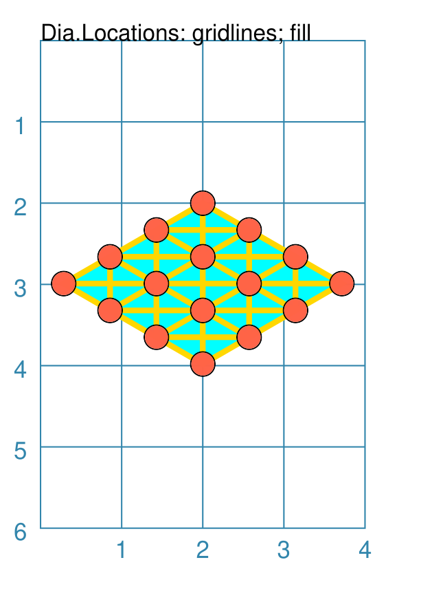
Example 10. Gridlines - Fill
|
This example shows the shape constructed using differing values for its properties. small_circle = circle(
radius=0.15,
fill="tomato")
dia = DiamondLocations(
facing='north',
y=2, x=2,
side=.66, cols=7)
Layout(
dia,
gridlines='*',
gridlines_fill="aqua",
gridlines_stroke="gold",
gridlines_stroke_width=2,
shapes=[small_circle])
Here, the grid itself is displayed — it is always drawn first before any shapes. The outline of the grid is always drawn. If the gridlines_fill property is assigned a color, then the grid will be filled with that color before any gridlines are drawn. The key prefix is gridlines and the value assigned to it will
determine in which direction, or directions, the gridlines are drawn;
in this case, because of the The usual customisation settings are possible for the gridlines; color, thickness, etc. |