Customised Shapes
The descriptions here assume you are familiar with the concepts, terms and ideas for protograf as presented in the Basic Concepts — especially units, properties and defaults.
You should have already seen how these shapes were created, with defaults, in Core Shapes.
However, while all shapes can be customised to some extent, and share some customisation options, these shapes in particular provide many more options which are described here.
Overview
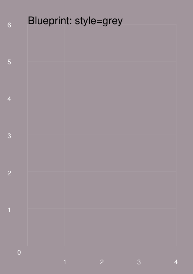
To make it easier to see where and how a shape has been drawn, most of these examples have been created with a background grid (which protograf refers to as a Blueprint shape) added to the page — a small A8 “business card” size — for cross-reference. In addition, the default Blueprint line width (aka stroke_width) has been made thicker for easier viewing of the small PNG images that were generated from the original PDF output.
A number of examples also use the Common command — this allows shared properties to be defined once and then used by any number of shapes.
Blueprint
This shape is primarily intended to support drawing while it is “in progress”.
It can take on the appearance of typical “cutting board”, so it provides a quick and convenient way to orientate and place other shapes that are required for the final product.
Typically one would just comment out the Blueprint command when its purpose has been served.
Blueprint Properties
In addition to the basic line styling properties, a Blueprint can also be customised with the following properties:
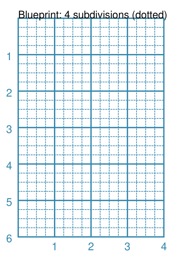
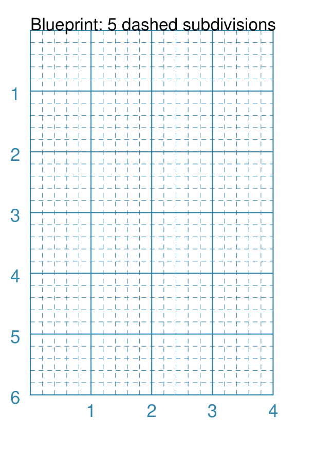
subdivisions - a number indicating how many lines should be drawn within each square; these are evenly spaces; use subdivisions_dashed to enhance these lines
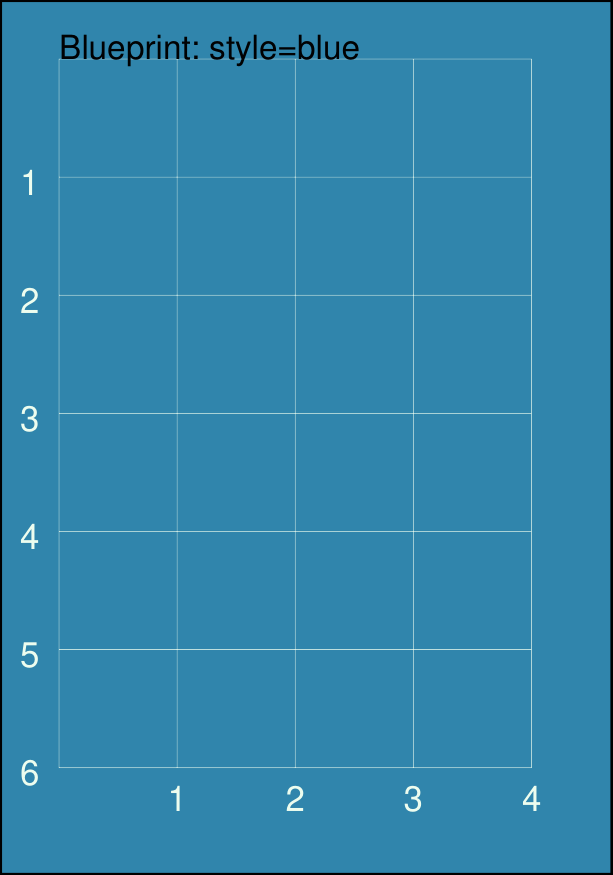
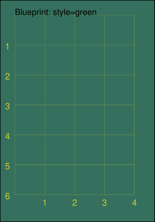
style - set to one of: blue, green or grey
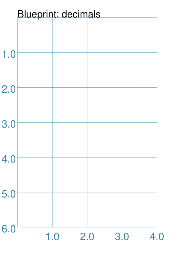
decimals - set to to an integer number for the decimal points which are used for the grid numbers (default is
0)edges - can be set to any combination of n, s, e, or w in a single comma-delimited string; grid numbers will then be drawn on any of the edges specified
edges_y - the number set for this determines where a horizontal line of grid numbers will be drawn
edges_x - the number set for this determines where a vertical line of grid numbers will be drawn
Examples showing how the Blueprint can be styled are described below.
Subdivisions
|
This example shows the Blueprint constructed using the command with these properties:
It has the following properties set:
Note subdivisions are not numbered and are automatically drawn with a thinner line in a dotted style. |
Subdivisions - Dashed
|
This example shows the Blueprint constructed using the command with these properties:
It has the following properties set:
Note subdivisions are not numbered and are automatically drawn with a thinner line using the dash settings. |
Style - Blue
|
This example shows the Blueprint constructed using the command with these properties:
It has the following properties set:
|
Style - Green
|
This example shows the Blueprint constructed using the command with these properties:
It has the following properties set:
|
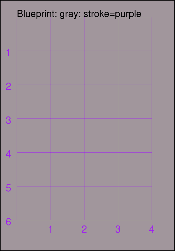
Style - Gray
|
This example shows the Blueprint constructed using the command with these properties:
It has the following properties set:
|
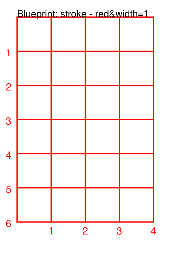
Stroke
|
This example shows the Blueprint constructed using the command with these properties:
It has the following properties set:
|
Fill
|
This example shows the Blueprint constructed using the command with these properties:
It has the following properties set:
Note: changes to line stroke, and line and fill color, will override the defaults for a chosen style. |
Decimals
|
This example shows the Blueprint constructed using the command with these properties:
It has the following properties set:
|
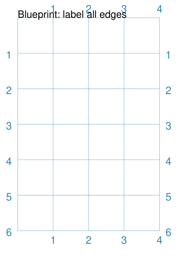
Edge Numbering
|
This example shows the Blueprint constructed using the command with these properties:
It has the following properties set:
Choose which edges should be numbered by using them in the list;
e.g. |
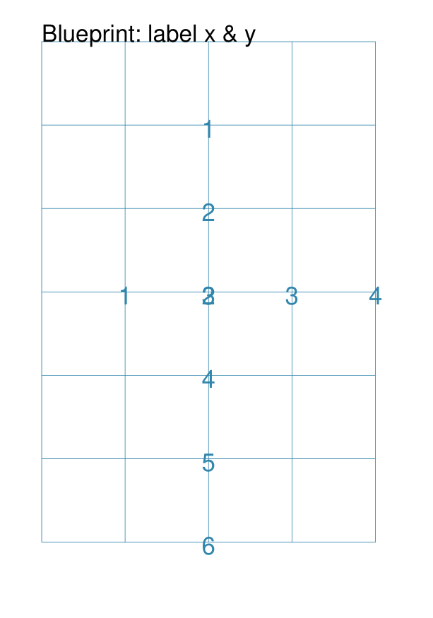
Edges Numbering at x and y
|
This example shows the Blueprint constructed using the command with these properties:
It has the following properties set:
This is not very useful for a tiny grid, but for a very large page size it can be helpful to set (or reset) such grid numbering while working on a complex design. |
Line
A Line is a very common shape in many designs; there are a number of ways that it can be customised.
Line Properties
A Line has the following properties, in addition to the basic ones of x and y for the starting point, and its label properties.
angle - the number of degrees clockwise that the line is rotated from the baseline about its start point; used in conjunction with length
curve - the distance from the centre point of the line through which a curve, joining the start and end of the line, must pass
cx and cy - if set, will replace the use of x and y for the starting point, and work in conjunction with angle and length to create the line around a centre point
centre_shapes - a list of one or more shapes that will be drawn at the centre of the line
centre_shapes_rotated - if set to
True, the shapes that will be drawn at the centre of the line are rotated to align with itdotted - if
True, create a series of small lines i.e. the “dots”, followed by gaps, of sizes equal to the line’s stroke_widthdashed - a list of two numbers: the first is the length of the dash; the second is the length of the space between each dash
length - sets the specific size of the line; used in conjunction with angle (which defaults to 0°)
links - a list of one or more shapes that will be joined by the line; this property overrides any others that may have been set to determine where the line is drawn
links_style - if set to
spoke, will draw lines from the first shape to each of the other shapes in the links listrounded - if
True, draw small circles, centred at the ends of the linesquared - if
True, draw small squares, centred at the ends of the linestroke - the color of the line
stroke_width - the thickness of the line, in points
wave_style - can be set to
'wave'or'sawtooth'wave_height - a numeric value for the height of each wave’s “peak”
x1 and y1 - a fixed endpoint for the line end (if not calculated by angle and length)
In addition, a line can have arrows at either or both ends. See the details in the arrowheads example.
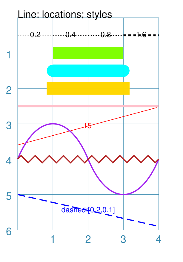
Example 1a. Dotted, Dashed, Angled and Wavy Lines
|
This example shows a Line constructed using commands with the following properties: # black lines
Line(
x=0, y=0.5,
stroke_width=0.2,
dotted=True,
label="0.2", font_size=6)
Line(
x=1, y=0.5,
stroke_width=0.4, dotted=True,
label="0.4", font_size=6)
Line(
x=2, y=0.5,
stroke_width=0.8, dotted=True,
label="0.8", font_size=6)
Line(
x=3, y=0.5,
stroke_width=1.6, dotted=True,
label="1.6", font_size=6)
# thick colored lines
Line(
x=1, y=1, stroke_width=10,
length=2, stroke="chartreuse")
Line(
x=1, y=1.5, stroke_width=10,
length=2, stroke="aqua",
stroke_ends="rounded")
Line(
x=1, y=2, stroke_width=10,
length=2, stroke="gold",
stroke_ends="squared")
# thin colored lines
Line(
x=0, y=5, x1=4, y1=5.9,
stroke="blue", stroke_width=1,
dashed=[0.2, 0.1],
label="dashed:[0.2,0.1]",
font_size=6)
Line(
x=0, y=3.6,
length=4.1, angle=15,
stroke="red",
label="15", font_size=6)
Line(
x=0, y=2.5, length=4,
stroke="pink", stroke_width=2)
# wavy lines
Line(
x=0, y=4, x1=4, y1=4,
stroke="purple", stroke_width=1,
wave_style='wave', wave_height=1.9)
Line(
x=0, y=4, x1=4, y1=4,
stroke="firebrick", stroke_width=1,
wave_style='sawtooth', wave_height=0.1)
The various black lines have these properties:
The dotted line is just a series of small lines i.e. all of the “dots”, followed by gaps, are of sizes equal to the line’s stroke_width. The thin, bright red line has:
The angle guides the direction in which the line is drawn; if not given — as in the case of most of the other lines — this will be 0°. The line length is then calculated based on these points. The green, gold, pink, bright red and aqua lines all have:
The thick green, gold, aqua and pink lines do not have any angle property; this defaults to 0° which means the line is drawn to the “east” (or right of the start). The thick aqua line has:
The thick gold line has:
The dark blue line has:
Dashes are a list of two numbers. The first is the length of the dash; the second is the length of the space between each dash. The purple line has:
The dark red line has:
|
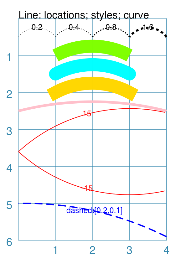
Example 1b. Dotted, Dashed and Angled Lines - curved
|
This example shows a Line constructed using commands with the following properties: # black lines
Line(
x=0, y=0.5,
stroke_width=0.2,
dotted=True,
label="0.2", font_size=6,
curve=0.25)
Line(
x=1, y=0.5,
stroke_width=0.4, dotted=True,
label="0.4", font_size=6,
curve=0.25)
Line(
x=2, y=0.5,
stroke_width=0.8, dotted=True,
label="0.8", font_size=6,
curve=0.25)
Line(
x=3, y=0.5,
stroke_width=1.6, dotted=True,
label="1.6", font_size=6,
curve=0.25)
# thick colored lines
Line(
x=1, y=1, stroke_width=10,
length=2, stroke="chartreuse",
curve=0.25)
Line(
x=1, y=1.5, stroke_width=10,
length=2, stroke="aqua",
stroke_ends="rounded",
curve=0.25)
Line(
x=1, y=2, stroke_width=10,
length=2, stroke="gold",
stroke_ends="squared",
curve=0.25)
# thin colored lines
Line(
x=0, y=5, x1=4, y1=5.9,
stroke="blue", stroke_width=1,
dashed=[0.2, 0.1],
label="dashed:[0.2,0.1]",
font_size=6,
curve=0.25)
Line(
x=0, y=3.6,
length=4.1, angle=15,
stroke="red",
label="15",
font_size=6,
curve=0.25)
Line(
x=0, y=2.5, length=4,
stroke="pink",
stroke_width=2,
curve=0.25)
This example is almost exactly the same as the one above Example 1a. Dotted, Dashed, Angled and Wavy Lines but with two key changes.
For more on curves, see Example 2. Curved Line. |
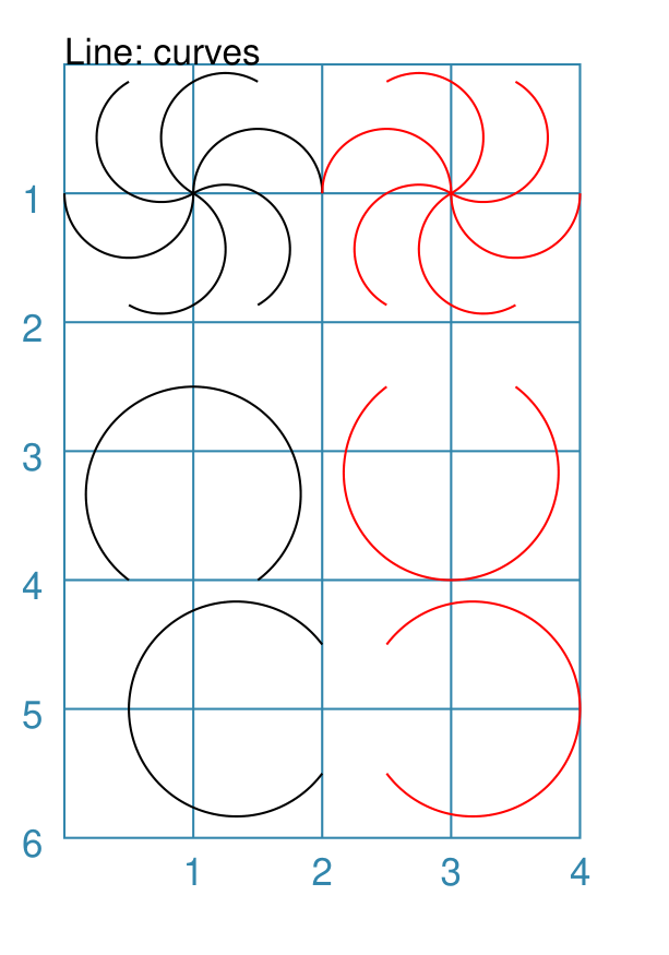
Example 2. Curved Line
A line can be drawn as a curve by providing a value for the curve property.
The curve value represents the distance above, or below if the value is negative, the centre point of the line through which the curve must pass; the curve is calculated as the arc of a circle joining the start, the “elevated centre” and the end of the line.
|
This example shows a Line constructed using commands with the following properties: tl = Common(
x=1, y=1,
length=1, curve=0.5)
Line(common=tl, angle=60)
Line(common=tl, angle=120)
Line(common=tl, angle=180)
Line(common=tl, angle=240)
Line(common=tl, angle=300)
Line(common=tl, angle=360)
tr = Common(
x=3, y=1, length=1,
curve=-0.5, stroke="red")
Line(common=tr, angle=60)
Line(common=tr, angle=120)
Line(common=tr, angle=180)
Line(common=tr, angle=240)
Line(common=tr, angle=300)
Line(common=tr, angle=360)
Line(
x=0.5, y=4,
length=1, curve=1.5)
Line(
x=2.5, y=2.5,
stroke="red",
length=1, curve=-1.5)
Line(
x=2, y=5.5, angle=90,
length=1, curve=1.5)
Line(
x=2.5, y=5.5, angle=90,
stroke="red",
length=1, curve=-1.5)
Here, the lines in the top-third of the drawing represent curved lines drawn at various angles; the black lines on left side show a positive curve, with lines curving “up” and the red lines on right side show a negative curve, with lines curving “down”. The lines in the lower section shows how the curve approaches the shape of a circle as the curve value increases. Again, black lines represent a “positive” curve and red lines represent a “negative” curve. |
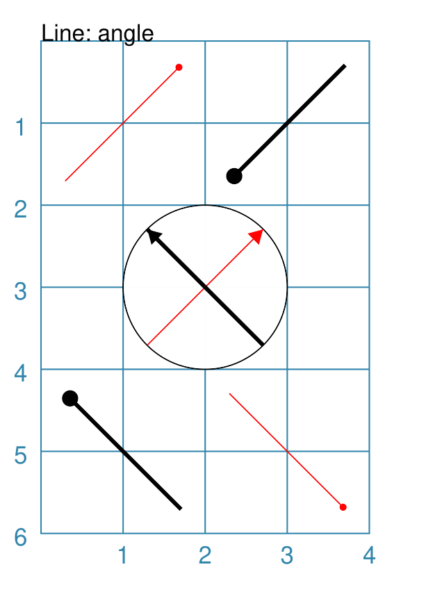
Example 3. Centred Line
A line can be drawn at a centre point by providing the following properties:
centre - set using cx and cy values
length - the length of the line
angle - the rotation of the line, anti-clockwise from the baseline
|
This example shows a Line constructed using commands with the following properties: Line(cx=1, cy=1, angle=45,
length=2, stroke="red",
arrow_style="circle")
Line(cx=3, cy=1, angle=225,
length=2, stroke_width=1.5,
arrow_style="c",
arrow_width=0.2)
Circle(cx=2, cy=3, radius=1)
Line(cx=2, cy=3, angle=45, length=2,
stroke="red", arrow_width=0.2)
Line(cx=2, cy=3, angle=135, length=2,
stroke_width=1.5, arrow_width=0.2)
Line(cx=1, cy=5, angle=135,
length=2, stroke_width=1.5
arrow_style="circle",
arrow_width=0.2)
Line(cx=3, cy=5, angle=315,
length=2, stroke="red",
arrow_style="c")
The top two lines are rotated at 45° (red) and 255° (thick black). The direction of rotation is shown by the circular “arrowhead” at the end of each line. The bottom two lines are rotated at 135° (thick black) and 315° (red). The direction of rotation is shown by the circular “arrowhead” at the end of each line. While each of the red/black pairs appear to be “in the same direction” — or parallel — the use of the arrow property displays the actual direction. Similarly, in the circle, 45° (red) line in the circle points north-east, while the 135° (thick black) points to north-west. For more on use of arrowheads, see Example 4. Arrowheads on Line. |
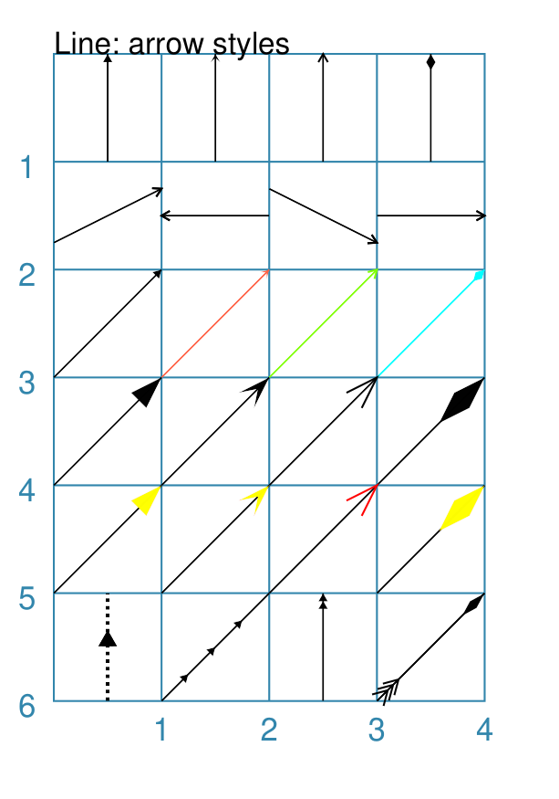
Example 4. Arrowheads on Line
In addition to styling a Line, it is also possible to specify an arrow (also called an “arrowhead”) for the line; a small “pointing” symbol to signify direction.
This is different from the standalone Arrow which allows a much higher degree of customisation and styling.
The following properties can be set:
arrow - if set to
Truewill cause a default arrow to be drawnarrow_style - can be set to
notch,angle,circle, orspearto change the default shape of the arrowarrow_fill - set the color of the arrow, which otherwise defaults to the color of the line
arrow_stroke - set the color of the arrow with style
angle, which otherwise defaults to the color of the linearrow_width - set the width of the arrow at its base, which otherwise defaults to a multiple of the line width — it also sets the radius of the arrow if its shape is circular
arrow_height - set the height of the arrow, which otherwise defaults to a value proportional to the arrow width — specifically, the height of the equilateral triangle used for the default arrow style
arrow_position - set a value (single number), or values (list of numbers), that represents the fractional distance along the line at which the arrow tip, or tips, must be positioned relative to the start of the line
arrow_double - if set to
Truemake a copy of the same arrow, with the same properties as above, but facing in the opposite direction
|
This example shows a Line constructed using commands with the various properties. Note the use of the Common command for when multiple Lines all need to share the same properties. # black styled arrows
Line(x=0.5, y=1, x1=0.5, y1=0,
arrow=True)
Line(x=1.5, y=1, x1=1.5, y1=0,
arrow_style='notch')
Line(x=2.5, y=1, x1=2.5, y1=0,
arrow_style='angle')
Line(x=3.5, y=1, x1=3.5, y1=0,
arrow_style='spear')
# rotated lines; double arrow
dbl_ang = Common(
arrow_style='angle',
arrow_double=True)
Line(common=dbl_ang,
x=0, y=1.75, x1=1, y1=1.25)
Line(common=dbl_ang,
x=2, y=1.5, x1=1, y1=1.5)
Line(common=dbl_ang,
x=2, y=1.25, x1=3, y1=1.75)
Line(common=dbl_ang,
x=3, y=1.5, x1=4, y1=1.5)
# colored lines and arrows
Line(x=0, y=3, x1=1, y1=2,
arrow=True)
Line(x=1, y=3, x1=2, y1=2,
arrow_style='notch',
stroke="tomato")
Line(x=2, y=3, x1=3, y1=2,
arrow_style='angle',
stroke="chartreuse")
Line(x=3, y=3, x1=4, y1=2,
arrow_style='spear',
stroke="aqua")
# set size of arrow heads
bigger = Common(
arrow_width=0.2,
arrow_height=0.3)
Line(common=bigger,
x=0, y=4, x1=1, y1=3,)
Line(common=bigger,
x=1, y=4, x1=2, y1=3,
arrow_style='notch')
Line(common=bigger,
x=2, y=4, x1=3, y1=3,
arrow_style='angle')
Line(common=bigger,
x=3, y=4, x1=4, y1=3,
arrow_style='spear')
# sized and colored arrow heads
big_color = Common(
arrow_width=0.2,
arrow_height=0.3,
arrow_fill="yellow",
arrow_stroke="red")
Line(common=big_color,
x=0, y=5, x1=1, y1=4,)
Line(common=big_color,
x=1, y=5, x1=2, y1=4,
arrow_style='notch')
Line(common=big_color,
x=2, y=5, x1=3, y1=4,
arrow_style='angle')
Line(common=big_color,
x=3, y=5, x1=4, y1=4,
arrow_style='spear')
# positioned arrow heads
Line(x=0.5, y=6, x1=0.5, y1=5,
stroke_width=1,
dotted=True,
arrow_position=0.66,
arrow_double=True)
Line(x=1, y=6, x1=2, y1=5,
arrow_position=[0.25, 0.5, 0.75])
Line(x=2.5, y=6, x1=2.5, y1=5,
arrow_position=[1.0, 0.93])
# two lines superimposed
Line(x=3, y=6, x1=4, y1=5,
arrow_style='spear',
arrow_height=0.15)
Line(x=3, y=6, x1=4, y1=5,
arrow_style='angle',
arrow_width=0.15,
arrow_position=[0.1, 0.15, 0.2])
The first row shows default-sized arrows of differing styles;
To enable an arrow display, either use The second row shows the default arrow but with the line rotated in
different directions. In this case The third row shows how arrows take on the stroke color of the line to which they are attached. The fourth row shows how the arrow’s height and width (across the
“base” of the arrow) can be set to control it’s size. Note that the
The fifth row shows how the arrow can be set to a different color from
that of its line. Note that the The sixth row shows how the arrow_position property can be set. The
value, or values, represent the fractional distance along the line at
which the arrow tip, or tips, is positioned relative to the start of
the line. So, The bottom left image shows how the default arrow expands in size
proportional to the thickness (stroke_width) of the line. Again,
because The bottom right image is a “cheat” of sorts. Two lines are drawn in the same location but with different styled arrows in different positions. An example of a circle arrowhead is shown in Example 3. Centred Line |
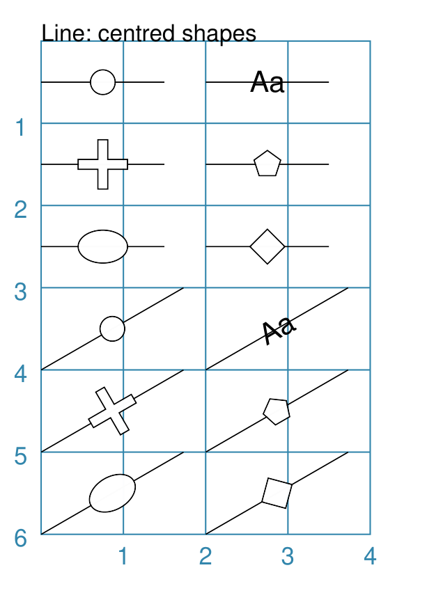
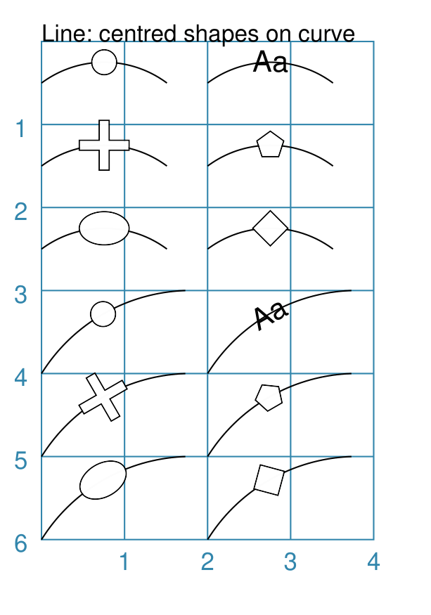
Example 5a. Centre Shapes
|
This example shows Lines constructed using commands with the following properties: crc = circle(radius=0.15)
ttt = text("Aa", font_size=10)
crs = cross(height=0.6, width=0.6)
ell = ellipse(height=0.4, width=0.6)
ply = polygon(side=0.2, sides=5)
rho = rhombus(side=0.3)
Line(x=0, y=0.5, length=1.5,
centre_shapes=[crc])
Line(x=2, y=0.5, length=1.5,
centre_shapes=[ttt])
Line(x=0, y=1.5, length=1.5,
centre_shapes=[crs])
Line(x=2, y=1.5, length=1.5,
centre_shapes=[ply])
Line(x=0, y=2.5, length=1.5,
centre_shapes=[ell])
Line(x=2, y=2.5, length=1.5,
centre_shapes=[rho])
Line(x=0, y=4, length=2,
angle=30,
centre_shapes=[crc],
centre_shapes_rotated=True)
Line(x=2, y=4, length=2,
angle=30,
centre_shapes=[ttt],
centre_shapes_rotated=True)
Line(x=0, y=5, length=2,
angle=30,
centre_shapes=[crs],
centre_shapes_rotated=True)
Line(x=2, y=5, length=2,
angle=30,
centre_shapes=[ply],
centre_shapes_rotated=True)
Line(x=0, y=6, length=2,
angle=30,
centre_shapes=[ell],
centre_shapes_rotated=True)
Line(x=2, y=6, length=2,
angle=30,
centre_shapes=[rho],
centre_shapes_rotated=True)
This example shows how shapes can placed on a line, such that the centre of the shapes are automatically at the line’s centre point. The centre_shapes property is set to a list ( If the shape should be rotated in the same direction as the line, then
the centre_shapes_rotated property should be set to |
Example 5b. Centre Shapes - curve
|
This example shows Lines constructed using commands with the following properties: crc = circle(radius=0.15)
ttt = text("Aa", font_size=10)
crs = cross(height=0.6, width=0.6)
ell = ellipse(height=0.4, width=0.6)
ply = polygon(side=0.2, sides=5)
rho = rhombus(side=0.3)
shrt = Common(length=1.51, curve=0.25)
Line(x=0, y=0.5, common=shrt,
centre_shapes=[crc])
Line(x=2, y=0.5, common=shrt,
centre_shapes=[ttt])
Line(x=0, y=1.5, common=shrt,
centre_shapes=[crs])
Line(x=2, y=1.5, common=shrt,
centre_shapes=[ply])
Line(x=0, y=2.5, common=shrt,
centre_shapes=[ell])
Line(x=2, y=2.5, common=shrt,
centre_shapes=[rho])
lng = Common(length=2, curve=0.25)
Line(x=0, y=4, common=lng,
angle=30,
centre_shapes=[crc],
centre_shapes_rotated =True)
Line(x=2, y=4, common=lng,
angle=30,
centre_shapes=[ttt],
centre_shapes_rotated =True)
Line(x=0, y=5, common=lng,
angle=30,
centre_shapes=[crs],
centre_shapes_rotated =True)
Line(x=2, y=5, common=lng, angle=30,
centre_shapes=[ply],
centre_shapes_rotated =True)
Line(x=0, y=6, common=lng, angle=30,
centre_shapes=[ell],
centre_shapes_rotated =True)
Line(x=2, y=6, common=lng,
angle=30,
centre_shapes=[rho],
centre_shapes_rotated =True)
This example is almost exactly the same as the one above Example 5a. Centre Shapes but with the addition of the curve property to each line. The value for the curve is set in each of the two |
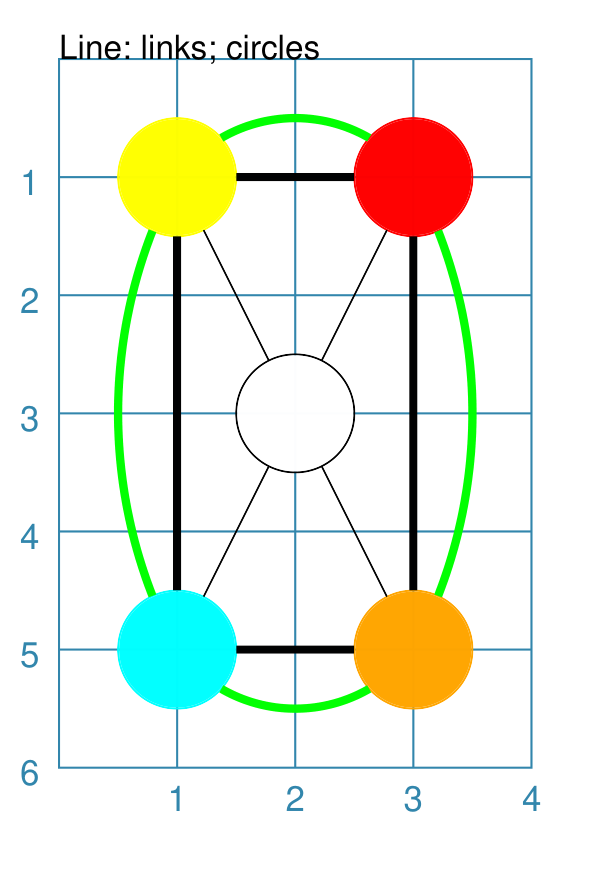
Example 6. Links: Circle
To link (or join or connect) two or more shapes, supply a list of them,
together with a link point, for the links property of a Line.
The link point for circular shapes — Circle and Dot —
is not required, as the connecting line is always drawn to/from the centre
of such a shape — but not crossing its boundary.
For non-circular shapes — for example, Rectangle or Hexagon —
such a shape must have either/or vertex points, or perbis points, that can be
specified as the link point to which the line will connect.
Note
Use of the links property overrides any other properties that may have been set to specify where the line will be drawn. The other properties that specify how the line will be appear will still be used.
|
This example shows a Line constructed using commands with the following properties: cc = Circle(cx=2, cy=3, radius=0.5)
cy = Circle(cx=1, cy=1, radius=0.5,
fill_stroke="yellow")
Line(links=[cc, cy])
ca = Circle(cx=1, cy=5, radius=0.5,
fill_stroke="aqua")
Line(links=[cc, ca])
cr = Circle(cx=3, cy=1,
radius=0.5, fill_stroke="red")
Line(links=[cc, cr])
co = Circle(cx=3, cy=5, radius=0.5,
fill_stroke="orange")
Line(links=[cc, co])
# orthogonal
Line(
links=[cy, cr, co, ca, cy],
stroke_width=2)
This example shows how Circles that are defined and drawn as normal
can be assigned to a name e.g. The links property requires two or more shapes in a list so that the Line can be drawn between them. Using the links property means that the normal point locations, or line angle, are not used but are superceded by calculated values. The “start” of the line is at the centre of the first circular shape and the “end” of the line is at the centre of the second circular shape. However, the line itself is only drawn between the boundaries of those shapes. The thick black line is drawn between a series of shapes, starting and ending at the yellow circle. |
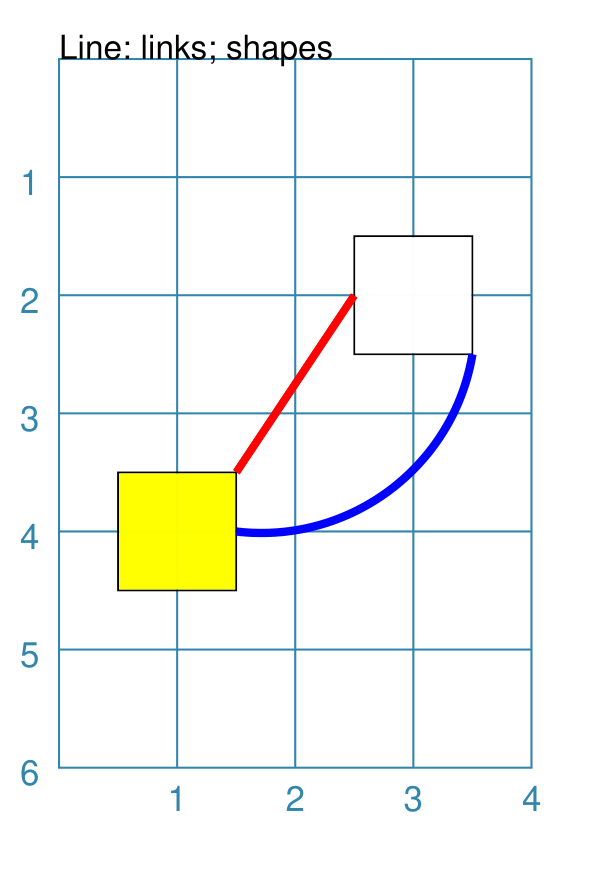
Example 7. Links: Shapes
To connect two or more non-circular shapes — for example, Rectangle
or Hexagon — supply a list of the link point of each ones, as
the links property of the line.
There are two ways to specify the link point setting for non-circular shapes.
The first option is the simpler — setting a point by relying on the
shape’s geometry. The point is specified using the
SHAPE.geo.DIR syntax; where SHAPE is the name assigned to the shape
by the script and POINT is the directional point name e.g. ne for a
north-east point.
The second option specifies a set of three values in this order:
the name assigned to the shape by the script;
the point type — either a vertex point (
v) or a perbis point (p);the link location, as a compass direction.
Note
Use of the links property overrides any other properties that may have been set to specify where the line will be drawn. The other properties that specify how the line will be appear will still be used.
More concrete examples of the use of links can be found in the board construction scripts — Morabaraba and Kensington.
|
This example shows a Line constructed using commands with the following properties: s1 = Square(
xx=1, cy=4, side=1,
fill="yellow")
s2 = Square(
cx=3, cy=2, side=1)
Line(
links=[s1.geo.ne, s2.geo.w],
stroke="red",
stroke_width=2)
Line(
links=[s1.geo.e, s2.geo.se],
stroke="blue",
stroke_width=2,
curve=-0.5)
This example shows how Squares that are defined and drawn as normal
can be assigned to a name e.g. The links property requires two or more shapes, together with their link points, in a list so that the Line can be drawn between them. Using the links property means that the normal point locations, or line angle, are not used but are superceded by the calculated values for the start and end of the line. In this case, for example, the start of the The |
Example 8. Links - Arrow
|
This example shows a Line constructed using commands with the following properties: cc = Circle(cx=1.5, cy=3.5, radius=0.5)
cy = Circle(cx=1, cy=1, radius=0.5,
fill_stroke="yellow")
co = Circle(cx=3, cy=5, radius=0.5,
fill_stroke="orange")
Line(links=[cy, cc, co],
stroke="red",
stroke_width=1,
arrow=True,
)
Similarly to Example 4, the line is drawn
between a series of In this case, the line has been styled with color and thickness, and the arrow has been “switched on”. The arrow points in the direction corresponding to the order of the shapes in the links list. |
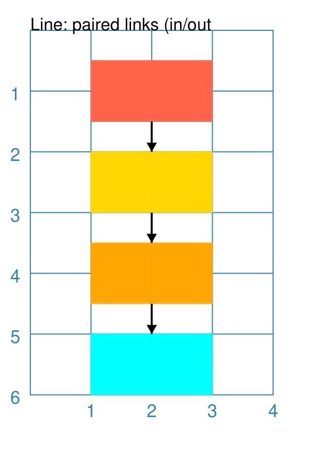
Example 9. Links - Pairs
|
This example shows a Line constructed using commands with the following properties: box = Common(x=1, height=1, width=2)
r1 = Rectangle(
common=box, y=0.5,
fill_stroke="tomato")
r2 = Rectangle(
common=box, y=r1.geo.nw + 1.5,
fill_stroke="gold")
r3 = Rectangle(
common=box, y=r2.geo.nw + 1.5,
fill_stroke="orange")
r4 = Rectangle(
common=box, y=r3.geo.nw + 1.5,
fill_stroke="aqua")
Line(
links=[r1.geo.s,
[r2.geo.n, r2.geo.s],
[r3.geo.n, r3.geo.s],
r4.geo.n],
stroke_width=1,
arrow=True)
In this example, lines, styled as arrows, are drawn between a series of
In this example, the “middle” boxes — yellow and orange — have
both incoming and outgoing arrows set by pairing the in and out points
for each rectangle together in a list, as shown by the square brackets
from |
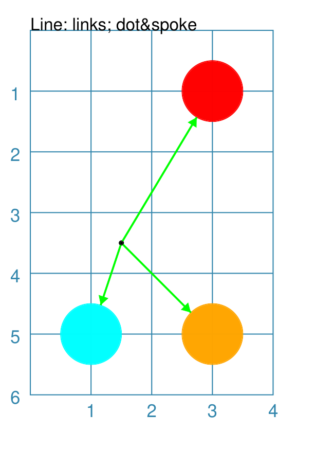
Example 10. Links - Spokes
|
This example shows a Line constructed using commands with the following properties: cc = Dot(cx=1.5, cy=3.5, dot_width=2)
cr = Circle(cx=3, cy=1, radius=0.5,
fill_stroke="red")
co = Circle(cx=3, cy=5, radius=0.5,
fill_stroke="orange")
ca = Circle(cx=1, cy=5, radius=0.5,
fill_stroke="aqua")
Line(links=[cc, cr, co, ca],
links_style='spoke',
stroke="green",
stroke_width=1,
arrow=True,
)
Similarly to Example 6, the line is drawn as an arrow between the shapes. However, the use of the Note that |
Example 11. Links - Curved
|
This example shows a Line constructed using commands with the following properties: cc = Dot(
cx=1.5, cy=3.5, dot_width=2)
cr = Circle(
cx=3, cy=1,
radius=0.5, fill_stroke="red")
co = Circle(
cx=3, cy=5,
radius=0.5, fill_stroke="orange")
ca = Circle(
cx=1, cy=5,
radius=0.5, fill_stroke="aqua")
Line(links=[cc, cr, co, ca],
links_style='spoke',
stroke="green",
stroke_width=1,
curve=0.5,
)
Here a “spoke” arrangement is created with the small black dot acting
as the central hub and curved lines — set by |

Rectangle
A Rectangle is a very common shape in many designs; there are a number of ways that it can be customised.
Centred
|
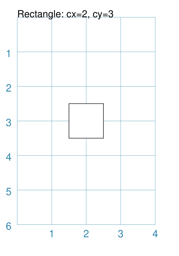
This example shows a Rectangle constructed using the command: Rectangle(cx=2, cy=3)
It has the following properties that differ from the defaults:
|
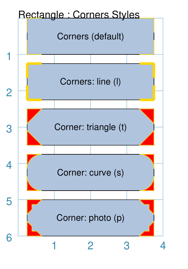
Corners
The corners property can superimpose a drawing onto each corner of the Rectangle. Each corner drawing can support customisation of its size, stroke color, fill color and style. The available styles are:
line - a simple line
triangle - a triangular shape
curve - a triangular shape with a curved inner edge
photo - a triangular shape with a cut-out notch
It is possible to limit where the corners are drawn by setting the
corner_directions property to one or more of the secondary compass
directions e.g. corner_directions="ne sw".
|
This example shows a Rectangle constructed using the command: styles = Common(
height=1, width=3.5, x=0.25,
label_size=7,
fill="lightsteelblue",
corner=0.4,
corner_stroke="gold",
corner_fill='red',
)
Rectangle(
common=styles, y=0,
label='Corner (default)')
Rectangle(
common=styles, y=1.25,
corner_style='line',
corner_stroke_width=2,
label='Corner: line (l)')
Rectangle(
common=styles, y=2.5,
corner_style='triangle',
label='Corner: triangle (t)')
Rectangle(
common=styles, y=3.75,
corner_style='curve',
label='Corner: curve (s)')
Rectangle(
common=styles, y=5,
corner_style='photo',
label='Corner: photo (p)')
Here all corners share a common stroke ( The default corner is a simple line, as shown in the top rectangle. |
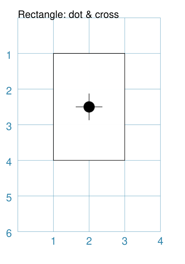
Cross and Dot
A cross or a dot are symbols that mark the centre of the Rectangle. They are usually the last parts that are drawn.
|
This example shows a Rectangle constructed using the command: Rectangle(height=3, width=2, cross=0.75, dot=0.15)
It has the following properties that differ from the defaults:
|
Chevron
A chevron converts opposite sides of the Rectangle into two triangular peaks that both point in a specified direction. This creates an arrow-like effect.
|
This example shows Rectangles constructed using these commands: styles = Common(
height=2, width=1,
font_size=4)
Rectangle(
common=styles,
x=3, y=2,
chevron='N',
chevron_height=0.5,
label="chevron:N:0.5",
title="title-N",
heading="head-N",
)
Rectangle(
x=0, y=2,
chevron='S',
chevron_height=0.5,
label="chevron:S:0.5",
title="title-S",
heading="head-S",
)
Rectangle(
x=1, y=4.5,
chevron='W',
chevron_height=0.5,
label="chevron:W:0.5",
title="title-W",
heading="head-W",
)
Rectangle(
x=1, y=0.5,
chevron='E',
chevron_height=0.5,
label="chevron:E:0.5",
title="title-E",
heading="head-E",
)
These Rectangles all share the following Common properties that differ from the defaults:
Each Rectangle has its own setting for:
Note that the label is centered in the Rectangle and not between the chevrons. |
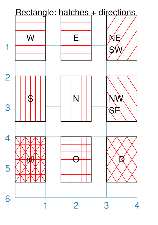
Hatches
Hatches are a set of parallel lines that are drawn, in a specified direction, across the length or width of the Rectangle in a vertical, horizontal or diagonal direction. Hatches are equally spaced across the height or width of the Rectangle.
|
This example shows Rectangles constructed using these commands: htch = Common(
height=1.5, width=1,
hatches_count=5,
hatches_stroke_width=0.1,
hatches_stroke="red")
Rectangle(
common=htch, x=0, y=0, hatches='w', label="W")
Rectangle(
common=htch, x=1.5, y=0, hatches='e', label="E")
Rectangle(
common=htch, x=3, y=0, hatches='ne', label="NE\nSW")
Rectangle(
common=htch, x=0, y=2, hatches='s', label="S")
Rectangle(
common=htch, x=1.5, y=2, hatches='n', label="N")
Rectangle(
common=htch, x=3, y=2, hatches='nw', label="NW\nSE")
Rectangle(
common=htch, x=0, y=4, label="all")
Rectangle(
common=htch, x=1.5, y=4, hatches='o', label="O")
Rectangle(
common=htch, x=3, y=4, hatches='d', label="D")
These Rectangles all share the following Common properties that differ from the defaults:
Each Rectangle has its own setting for:
|
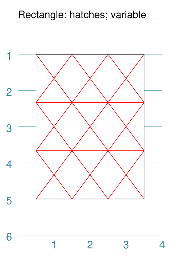
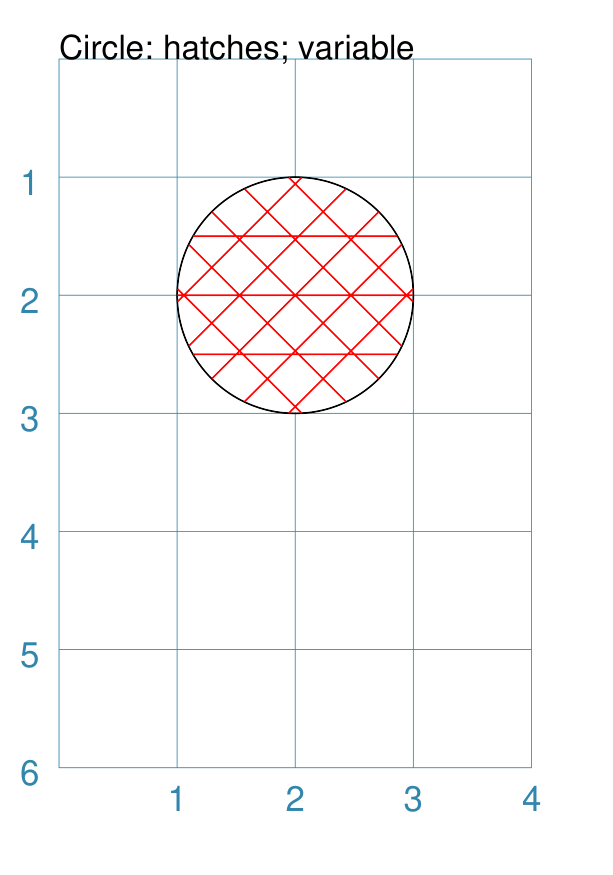
Hatches: Variable
As described in section on Hatches, these are normally spaced equally across the height or width of the Rectangle.
However it is possible to vary the number of hatch lines for any direction, or set of directions, by changing the setting for the hatches property.
This is illustrated in the example below.
|
This example shows a Rectangle constructed using these commands: Rectangle(
x=0.5, y=1,
height=4, width=3,
hatches=[('e', 2), ('d', 5)],
hatches_stroke_width=0.5,
hatches_stroke="red")
While other settings are similar to the previous example, in this
case the hatches property is in a list form, as shown by the square
brackets from
In this case, there are 2 lines in the |
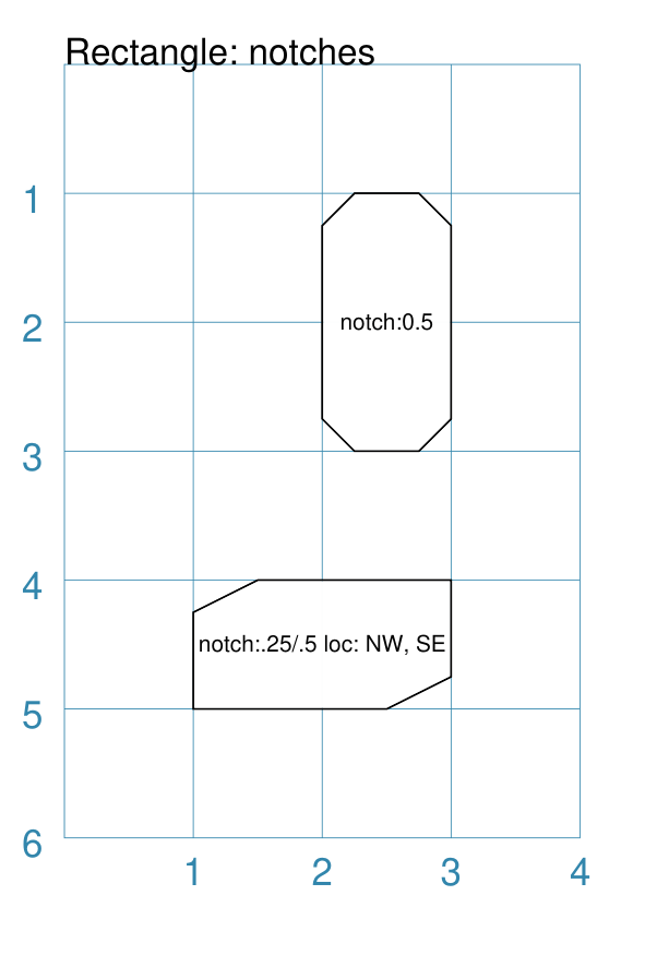
Notch
Notches are small indents — or outdents — that are drawn in the specified corners of the Rectangle.
Example 1. Size & Location
|
This example shows Rectangles constructed using these commands: Rectangle(
x=2, y=1, height=2, width=1,
label="notch:0.5", label_size=5,
notch=0.25,
)
Rectangle(
x=1, y=4, height=1, width=2,
label="notch:.25/.5 loc: NW, SE",
label_size=5,
notch_x=0.5, notch_y=0.25,
notch_directions="NW SE",
)
These share the following properties:
The first Rectangle has:
The second Rectangle has:
|
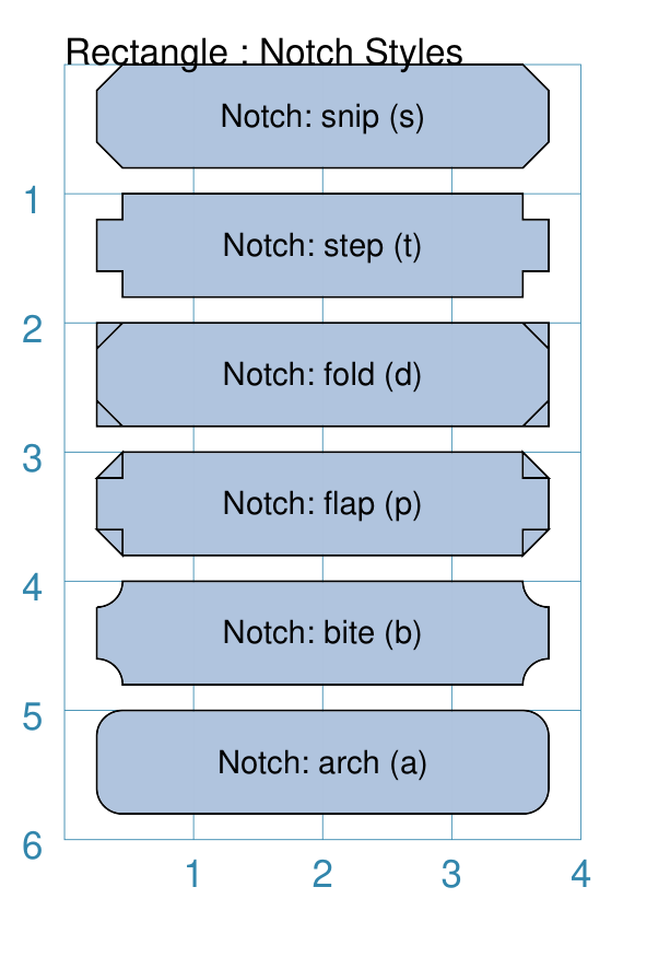
Example 2. Styles
|
These examples shows Rectangles constructed using these commands: styles = Common(
height=0.8, width=3.5, x=0.25,
notch=0.2, label_size=7,
fill="lightsteelblue")
Rectangle(
common=styles, y=0, notch_style='snip',
label='Notch: snip (s)')
Rectangle(
common=styles, y=1, notch_style='step',
label='Notch: step (t)')
Rectangle(
common=styles, y=2, notch_style='fold',
label='Notch: fold (o)')
Rectangle(
common=styles, y=3, notch_style='flap',
label='Notch: flap (l)')
Rectangle(
common=styles, y=4, notch_style='bite',
label='Notch: bite (b)')
Rectangle(
common=styles, y=5, notch_style='arch',
label='Notch: arch (a)')
These Rectangles all share the following Common properties that differ from the defaults:
Each notch_style results in a slightly different corner effect:
|
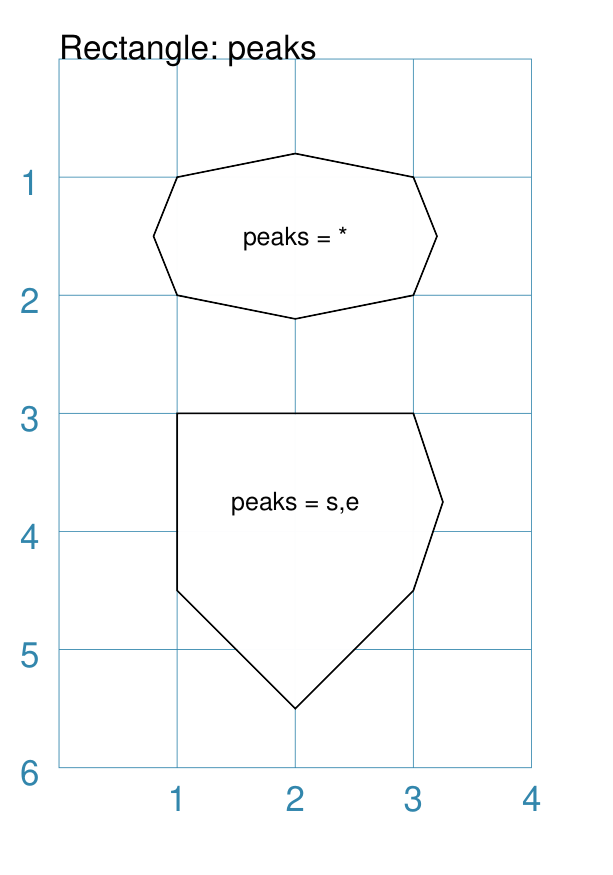
Peak
A peak is small triangular shape that juts out from the side of a Rectangle in a specified direction.
|
This example shows Rectangles constructed using these commands: Rectangle(
x=1, y=1, width=2, height=1,
font_size=6, label="peaks = *",
peaks=[("*", 0.2)]
)
Rectangle(
x=1, y=3, width=2, height=1,
font_size=6, label="points = s,e",
peaks=[("s", 1), ("e", 0.25)]
)
The Rectangles all have the following properties that differ from the defaults:
The peaks property is a list:
Note: If the value |
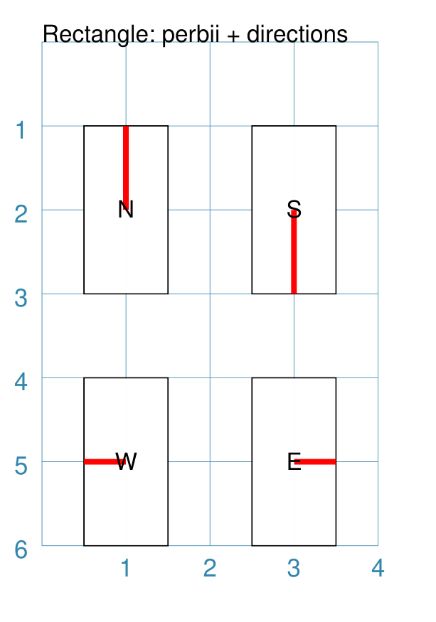
Perbii
“Perbis” is a shortcut name for “perpendicular bisector”; and “perbii” is the the plural. These lines are drawn from the centre of a Rectangle towards the mid-points of its edges.
|
This example shows Rectangles constructed using these commands: prbs = Common(
height=2, width=1,
perbii_stroke_width=2,
perbii_stroke="red")
Rectangle(
common=prbs, x=0.5, y=1,
perbii='n', label="N")
Rectangle(
common=prbs, x=2.5, y=1,
perbii='s', label="S")
Rectangle(
common=prbs, x=0.5, y=4,
perbii='w', label="W")
Rectangle(
common=prbs, x=2.5, y=4,
perbii='e', label="E")
These Rectangles all share the following Common properties that differ from the defaults:
Each Rectangle has its own setting for:
|
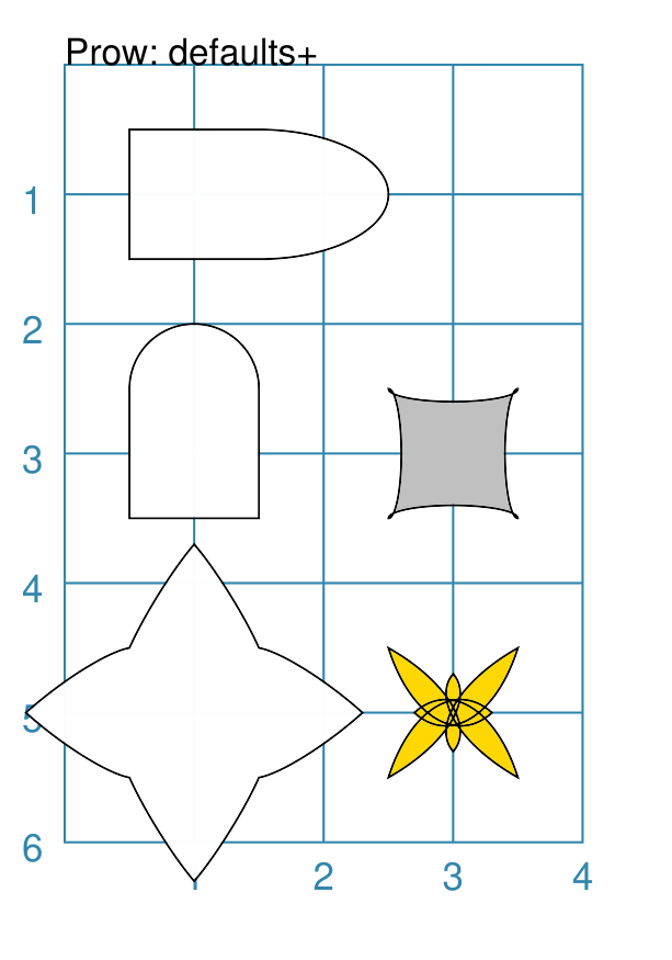
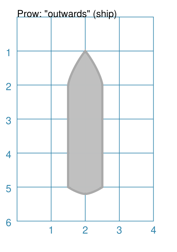
Prows
A prow is a pair of curved lines that jut out from the side of a Rectangle in a specified direction to a specifed distance.
The prow property is a list of one or more sets of values —
[(..), (...), ...].
Each set must start with a compass direction — n, s, e, or w —
indicating at which side the prow must be drawn. Using a value of "*"
means that the prow will be drawn in all directions.
The default prow will be two curves extending to a point 1 unit away
from the edge of the rectangle.
A set can also contain the prow height — the distance away from the from the edge of the rectangle.
Finally, a set can contain a pair of values that represent the positioning of a “control” point that will change the amount of the curvature of the prow lines. This pair is: the x distance relative to the perpendicular line through the centre of the edge; and the y distance relative to the edge — for top- and bottom edges; and vice-versa for the vertical edges. Both height and control values can be negative which will affect the direction of drawing.
Example 1. Defaults etc.
|
This example shows Rectangles constructed using these commands: Rectangle(
cx=1, cy=1, width=1, height=1,
prows=[("e",)]
)
Rectangle(
cx=1, cy=3, width=1, height=1,
prows=[("n", 0.5)]
)
Rectangle(
cx=3, cy=3, width=1, height=1,
fill="silver",
prows=[("*", -0.1)]
)
Rectangle(
cx=1, cy=5, width=1, height=1,
prows=[("*", 0.8, (0.3, 0.45))]
)
Rectangle(
cx=3, cy=5, width=1, height=1,
fill="gold",
prows=[("*", -0.8, (-0.3, -0.45))]
)
The top rectangle has a single prow extending in the east direction;
this has a default distance of The middle-left rectangle has a single prow extending in the north
direction; this has a specified distance of The bottom-left rectangle has prows extending in all directions ( The grey middle-right rectangle has a negative height of The yellow bottom-right rectangle has prows extending in all directions and negative height and negative control point values. This results in the unusual pattern shown. |
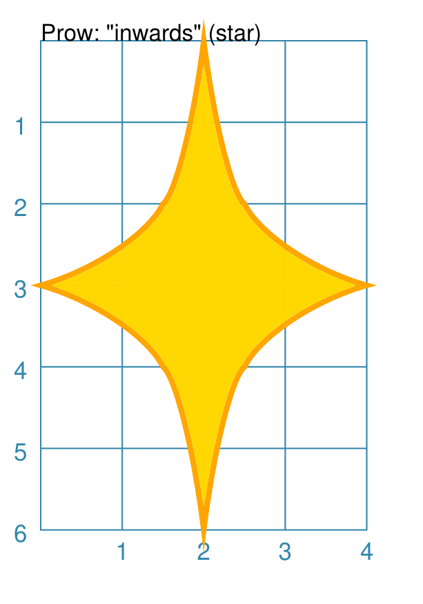
Example 2. Inwards
|
This example shows a Rectangle constructed using these properties: Rectangle(
x=1.5, y=2, width=1, height=2,
fill="gold",
stroke="orange",
stroke_width=2,
prows=[
("n", 2, (0.22, 0.22)),
("s", 2, (0.22, 0.22)),
("e", 1.5, (0.33, 0.33)),
("w", 1.5, (0.33, 0.33)),
]
)
This example shows how an almost-seamless star-like shape can be formed by appropriate setting of the control points for a rectangle. |
Example 3. Outwards
|
This example shows a Rectangle constructed using these properties: Rectangle(
x=1.5, y=2, width=1, height=3,
fill="silver",
stroke="darkgrey",
stroke_width=2,
prows=[
("n", 1, (0.44, 0.44)),
("s", 0.2, (0.2, 0.2)),
]
)
This example shows how a ship-like shape can be formed by appropriate setting of the heights and control points for a rectangle. |
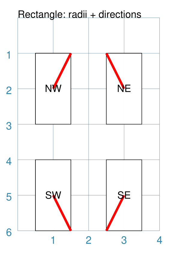
Radii
Radii are lines from the centre of a Rectangle towards its vertices.
|
This example shows Rectangles constructed using these commands: rds = Common(
height=2, width=1,
radii_stroke_width=2,
radii_stroke="red")
Rectangle(
common=rds, x=0.5, y=1,
radii='nw', label="NW")
Rectangle(
common=rds, x=2.5, y=1,
radii='ne', label="NE")
Rectangle(
common=rds, x=0.5, y=4,
radii='sw', label="SW")
Rectangle(
common=rds, x=2.5, y=4,
radii='se', label="SE")
These Rectangles all share the following Common properties that differ from the defaults:
Each Rectangle has its own setting for:
|
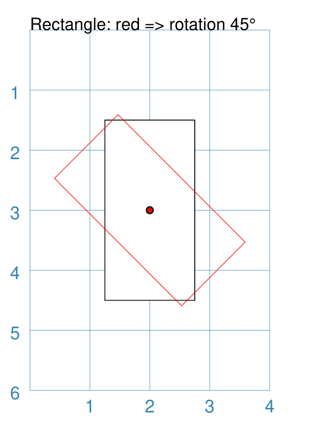
Rotation
Rotation takes place in anti-clockwise direction, from the horizontal, around the centre of the Rectangle.
|
This example shows Rectangles constructed using the commands: Rectangle(
cx=2, cy=3, width=1.5, height=3, dot=0.06)
Rectangle(
cx=2, cy=3, width=1.5, height=3, dot=0.04,
fill=None,
stroke="red", stroke_width=0.3, rotation=45,)
The first, upright, Rectangle is a normal one, with a black outline. It is centred at x-location The second Rectangle is similar to the first, except:
|
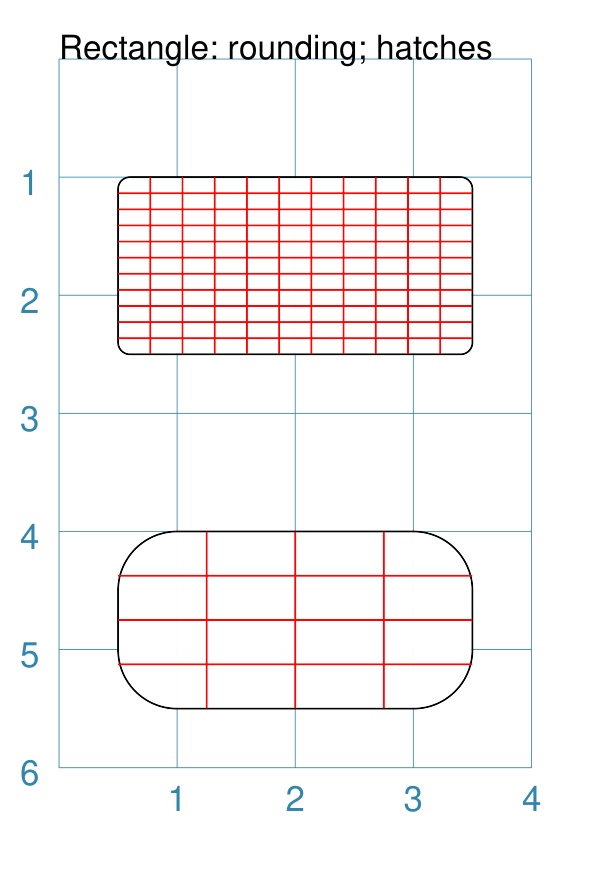
Rounding
Rounding changes the corners of a Rectangle from a sharp, right-angled, join into the arc of a quarter-circle.
|
This example shows Rectangles constructed using the commands: rct = Common(
x=0.5,
height=1.5, width=3.0,
stroke_width=.5,
hatches_stroke="red",
hatches='o')
Rectangle(
common=rct, y=1,
rounding=0.1,
hatches_count=10)
Rectangle(
common=rct, y=4,
rounding=0.5,
hatches_count=3)
Both Rectangles share the Common properties of:
These properties set the color and directions of the lines crossing the Rectangles. The upper Rectangle has these specific properties:
The lower Rectangle has these specific properties:
It should be noted that if the rounding is too large in comparison with the number of hatches, as in this example:
then the program will issue an error: No hatching permissible with this size rounding
|
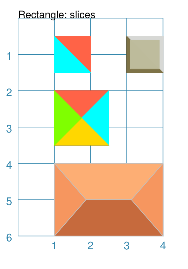
Slices
The slices-related command enables the Rectangle to be filled with colored triangular or quadilateral shapes.
Note
Slices are drawn after the rectangle has been drawn, and so may obscure the stroke outline and fill color of the rectangle.
|
This example shows Rectangles constructed using the commands: Rectangle(
x=1, y=0.5,
slices=['tomato', 'aqua'],
fill=None)
Rectangle(
x=3, y=0.5,
slices=['#D7D8D5', '#7E7347'],
fill=None,
centre_shape=square(
side=0.8, fill_stroke="#BEBC9D"))
Rectangle(
x=1, y=2,
height=1.5, width=1.5,
slices=['tomato', 'aqua', 'gold', 'chartreuse'],
fill=None)
Rectangle(
x=1, y=4,
height=2, width=3,
slices=['#FDAE74', '#F6965F', '#C66A3D', '#F6965F'],
slices_line=1.25,
slices_stroke="silver",
fill=None)
The top-left example shows the minimum required; the slices property is
a list of two colors ( The top-right example is similar to the top-left, but the addition of a centred square of intermediate color creates a “3D” effect. The middle example shows what happens when the slices property is given
a list of four colors ( The lower-most example shows what happens when the slices property is given a list of four colors, plus a slices_line and a slices_stroke. The slices_line is drawn centered in the rectangle, and then the two triangles are created at either end, with quadilaterals forming the top and bottom shapes. All lines are drawn with the slices_stroke color. |
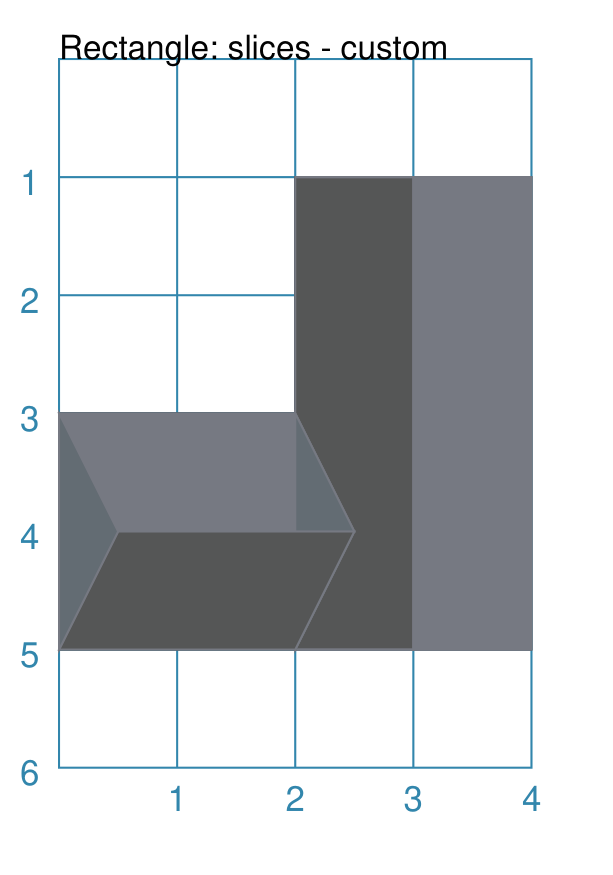
|
This example shows Rectangles constructed using the commands: Rectangle(
x=1, y=2,
height=2, width=4,
slices=['#555656', '#555656', '#767982', '#555656'],
slices_line=4,
slices_stroke="#767982",
rotation=90)
Rectangle(
x=0, y=3,
height=2, width=2,
slices=['#767982', '#636C73', '#555656', '#636C73'],
slices_line=2,
slices_stroke="#767982",
slices_line_mx=0.5)
Both examples shows what happens when the slices property is given
a list of four colors, plus a slices_line and a slices_stroke.
In both cases, the slices_line length is equal to the length of the
rectangle itself ( The right-hand rectangle shows how it appears to be subdivided into two areas; this is because the slices_line runs the full length of the rectangle so the end triangles have a height of zero and effectively become “invisible”. In addition, because the rectangle has been rotated by 90° (around its centre) the dividing line displays as vertical. The left-hand rectangle has an additional property slices_line_mx which causes the middle-line to move that distance to the right (or to the left, if it was a negative value). This causes the right-hand triangle to “project” to the right of the rectangle. |
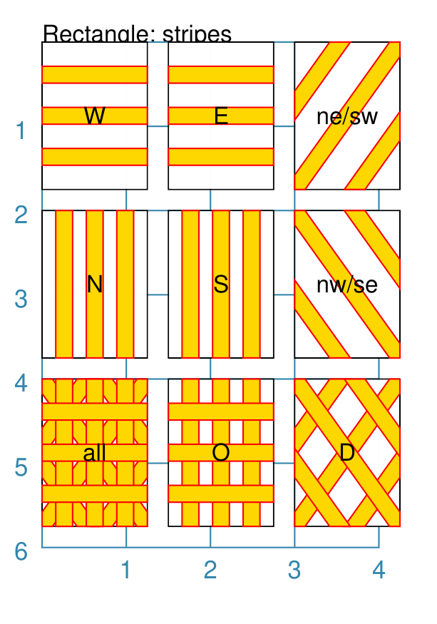
Stripes
Stripes are a set of equal-width parallel areas that are drawn, in a specified direction, across the length or width of the Rectangle in vertical, horizontal or diagonal directions.
The key properties to draw stripes are:
stripes - sets the number of stripes to be drawn; the intervals between them are calculated equally and depend on the direction and the breadth of the stripes
stripes_directions - sets the compass direction for the stripes to be drawn; defaults to
n(North)stripes_breadth - sets width of the stripe to be drawn; if not given, will be calculated to give 0a size that will result in equally sized stripes and gaps
In addition, the usual properties for stroke, stroke_width, fill and transparency can also be set.
|
This example shows Rectangles constructed using these commands: strp = Common(
height=1.75, width=1.25,
stripes=3,
stripes_breadth=0.2,
stripes_stroke="red",
stripes_fill="gold"
Rectangle(
common=strp, x=0, y=0,
stripes_directions='w', label="W")
Rectangle(
common=strp, x=1.5, y=0,
stripes_directions='e', label="E")
Rectangle(
common=strp, x=3, y=0,
stripes_directions='ne', label="NE\nSW")
Rectangle(
common=strp, x=0, y=2,
stripes_directions='s', label="S")
Rectangle(
common=strp, x=1.5, y=2,
stripes_directions='n', label="N")
Rectangle(
common=strp, x=3, y=2,
stripes_directions='nw', label="NW\nSE")
Rectangle(
common=strp, x=0, y=4,
stripes_directions='*',
label="all")
Rectangle(
common=strp, x=1.5, y=4,
stripes_directions='o', label="O")
Rectangle(
common=strp, x=3, y=4,
stripes_directions='d', label="D")
These Rectangles all share the following Common properties that differ from the defaults:
Each Rectangle has its own setting for:
|
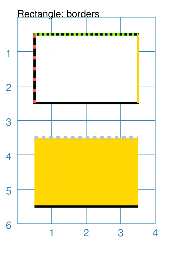
Borders
The Borders property allows for the normal line that is drawn around the
Rectangle to be overwritten on specific sides by another type of line.
The Borders property is specified by providing a set of values, which are
comma-separated inside round brackets, in the following order:
direction - one of (n)orth, (s)outh, (e)ast or (w)est
width - the line thickness
color - either a named color or a hexadecimal value
style -
Truemakes it dotted; or a list of values creates dashes
Direction and width are required, but color and style are optional. One
or more border values can be used together with spaces between them
e.g. n s to draw both lines on both north and south sides.
|
This example shows Rectangles constructed using these commands: Rectangle(
x=0.5, y=3.5,
height=2, width=3,
stroke=None, fill="gold",
borders=[
("n", 2, "lightsteelblue", True),
("s", 2),
]
)
Rectangle(
x=0.5, y=0.5,
height=2, width=3,
stroke_width=1.9,
borders=[
("w", 2, "gold"),
("n", 2, "chartreuse", True),
("e", 2, "tomato", [0.1, 0.2]),
]
)
The lower rectangle has a yellow fill but no stroke i.e. no lines are drawn around it. There are two borders that are set in the list (shown in
the square brackets going from
The top rectangle has a thick stroke_width as its outline, with a default fill of white and default stroke of black. There are three borders that are set in the list (the square brackets
going from
Note that for both dotted and dashed lines, any underlying color or image will “show though” the gaps in the line |
Ordering of Properties
There is a default order in which the various properties of a Rectangle are drawn. There are three ways to change this drawing order:
order_first - a list of properties that will be drawn, in the order given in the list, before any others
order_last - a list of properties that will be drawn, in the order given in the list, after any others
order_all - a list of the only properties that will be drawn, in the order given in the list
The available property names, shown in their default order, are:
base - this represents the Rectangle itself including those properties which control the way the edges are drawn; for example, the peak or prow settings
pattern
slices
stripes
hatches
radii
corners
radii_shapes
perbii_shapes
centre_shape
centre_shapes
vertex_shapes
dot
cross
text
numbering
Hexagon
A Hexagon is a regular, six-sided, polygon whose sides and interior angles are all equal.
A key property for a Hexagon is its orientation; this can either be flat, which is the default, with two opposing sides parallel to the top and bottom edges of the page or card, or pointy with two opposing sides parallel to the left and right edges of the page or card.
The examples below show how each orientation of a Hexagon can be customised in a similar way.
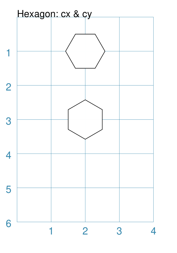
Centre
|
This example shows Hexagons constructed using these commands: Hexagon(cx=2, cy=1)
Hexagon(
cx=2, cy=3,
orientation='pointy')
Both Hexagons are positioned via their centres - cx and cy. The upper Hexagon has the default orientation value of The lower Hexagon also has the orientation property set to
|
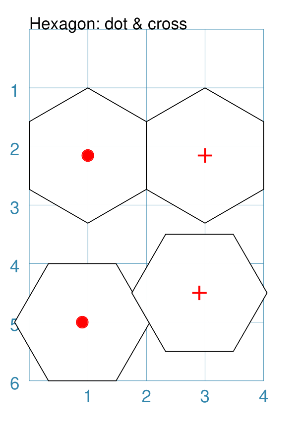
Dot & Cross
|
This example shows Hexagons constructed using these commands: Hexagon(
x=0, y=1, height=2,
dot=0.1, dot_stroke="red",
orientation='pointy')
Hexagon(
x=2, y=1, height=2,
cross=0.25, cross_stroke="red",
cross_stroke_width=1,
orientation='pointy')
Hexagon(
x=-0.25, y=4, height=2,
dot=0.1, dot_stroke="red")
Hexagon(
x=1.75, y=3.5, height=2,
cross=0.25, cross_stroke="red",
cross_stroke_width=1)
These Hexagons have properties set as follows:
|
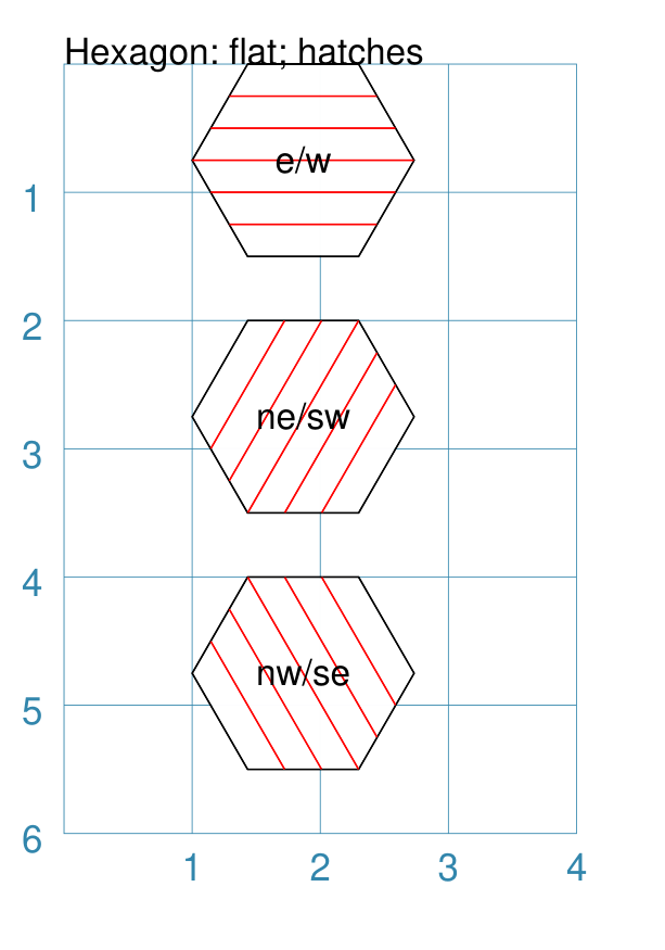
Hatches: Flat
Hatches are a set of parallel lines that are drawn across a Hexagon from one opposing side to another in a vertical, horizontal or diagonal direction. By default, hatches are equally spaced across the diameter of the Hexagon.
|
This example shows Hexagons constructed using these commands: hxgn = Common(
x=1, height=1.5, orientation='flat',
hatches_count=5, hatches_stroke="red")
Hexagon(
common=hxgn, y=0,
hatches='e', label="e/w")
Hexagon(
common=hxgn, y=2,
hatches='ne', label="ne/sw")
Hexagon(
common=hxgn, y=4,
hatches='nw', label="nw/se")
These Hexagons all share the following Common properties that differ from the defaults:
Each Hexagon has its own setting for:
|
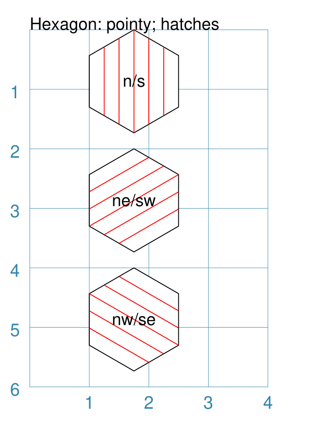
Hatches: Pointy
Hatches are a set of parallel lines that are drawn, in a specified direction, across the Hexagon from one opposing side to another in a vertical, horizontal or diagonal direction. By default, hatches are equally spaced across the diameter of the Hexagon.
|
This example shows Hexagons constructed using these commands: hxgn = Common(
x=1, height=1.5,
orientation='pointy',
hatches_count=5,
hatches_stroke="red")
Hexagon(
common=hxgn, y=0,
hatches='n', label="n/s")
Hexagon(
common=hxgn, y=2,
hatches='ne', label="ne/sw")
Hexagon(
common=hxgn, y=4,
hatches='nw', label="nw/se")
These Hexagons all share the following Common properties that differ from the defaults:
Each Hexagon has its own setting for:
|
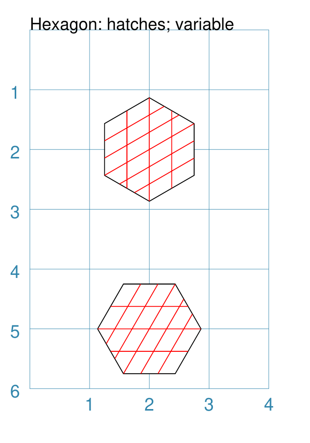
Hatches: Variable
As described in above, hatches are normally spaced equally across the sides of the Hexagon.
However it is possible to vary the number of hatch lines for any direction, or set of directions, by changing the setting for the hatches property.
|
This example shows the shape constructed using the command with the various properties. hhxgn = Common(
cx=2, height=1.5,
hatches_stroke="red")
Hexagon(
common=hhxgn, cy=2,
orientation='pointy',
hatches=[('s', 3), ('ne', 5)])
Hexagon(
common=hhxgn, cy=5,
orientation='flat',
hatches=[('w', 3), ('ne', 5)])
While other settings are similar to the previous example, in this
case the hatches property is in a list form, as shown by the square
brackets from
In the top example (“pointy” hex), there are 3 lines in the In the top example (“flat” hex), there are 3 lines in the |
Radii: Flat
Radii are like spokes of a bicycle wheel; they are drawn from the centre of a Hexagon towards its vertices.
|
This example shows Hexagons constructed using these commands: hxg = Common(
height=1.5, font_size=8,
dot=0.05,
dot_stroke="red",
orientation="flat")
Hexagon(
common=hxg, x=0.25, y=0.25,
radii='sw', label="SW")
Hexagon(
common=hxg, x=0.25, y=2.15,
radii='w', label="W")
Hexagon(
common=hxg, x=0.25, y=4,
radii='nw', label="NW")
Hexagon(
common=hxg, x=2.25, y=4,
radii='ne', label="NE")
Hexagon(
common=hxg, x=2.25, y=2.15,
radii='e', label="E")
Hexagon(
common=hxg, x=2.25, y=0.25,
radii='se', label="SE")
These have the following properties:
|
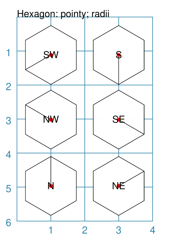
Radii: Pointy
Radii are like spokes of a bicycle wheel; they are drawn from the centre of a Hexagon towards its vertices.
|
This example shows Hexagons constructed using these commands: hxg = Common(
height=1.5, font_size=8,
dot=0.05, dot_stroke="red",
orientation="pointy")
Hexagon(
common=hxg, x=0.25, y=0.25,
radii='sw', label="SW")
Hexagon(
common=hxg, x=0.25, y=2.15,
radii='nw', label="NW")
Hexagon(
common=hxg, x=0.25, y=4,
radii='n', label="N")
Hexagon(
common=hxg, x=2.25, y=4,
radii='ne', label="NE")
Hexagon(
common=hxg, x=2.25, y=0.25,
radii='s', label="S")
Hexagon(
common=hxg, x=2.25, y=2.15,
radii='se', label="SE")
These have the following properties:
|
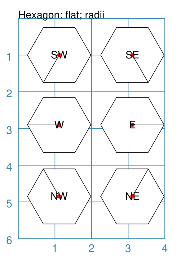
Perbii: Flat
“Perbis” is a shortcut name for a “perpendicular bisector”; and “perbii” is the the plural. These lines are like spokes of a bicycle wheel; they are drawn from the centre of a Hexagon towards the mid-points of the edges.
|
This example shows Hexagons constructed using these commands: hxg = Common(
height=1.5, font_size=8,
dot=0.05, dot_stroke="red",
orientation="flat")
Hexagon(
common=hxg, x=0.25, y=0.25,
perbii='sw', label="SW")
Hexagon(
common=hxg, x=0.25, y=2.15,
perbii='w', label="W")
Hexagon(
common=hxg, x=0.25, y=4,
perbii='nw', label="NW")
Hexagon(
common=hxg, x=2.25, y=4,
perbii='ne', label="NE")
Hexagon(
common=hxg, x=2.25, y=2.15,
perbii='e', label="E")
Hexagon(
common=hxg, x=2.25, y=0.25,
perbii='se', label="SE")
These have the following properties:
|
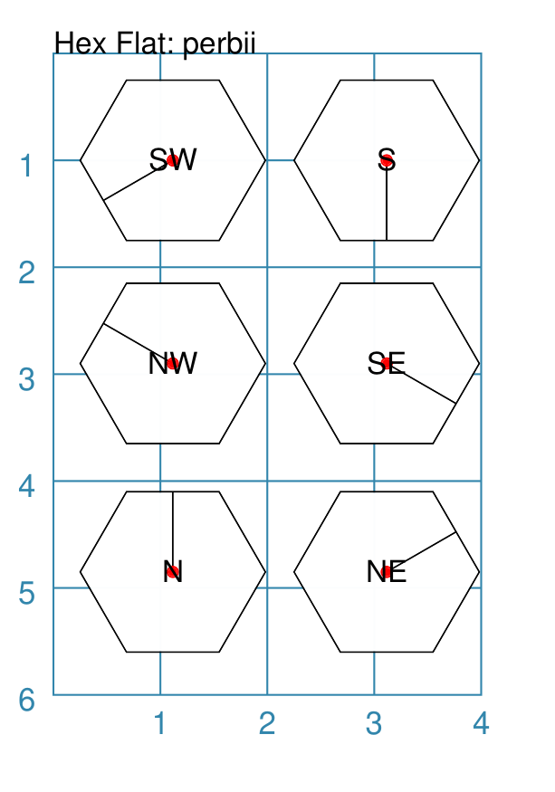
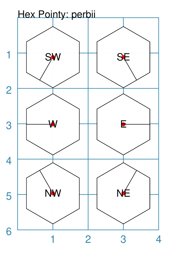
Perbii: Pointy
“Perbii” is a shortcut name for “perpendicular bisector”. These lines are like spokes of a bicycle wheel; they are drawn from the centre of a Hexagon towards the mid-points of the edges.
|
This example shows Hexagons constructed using these commands: hxg = Common(
height=1.5, font_size=8,
dot=0.05, dot_stroke="red",
orientation="pointy")
Hexagon(
common=hxg, x=0.25, y=0.25,
perbii='sw', label="SW")
Hexagon(
common=hxg, x=0.25, y=2.15,
perbii='nw', label="NW")
Hexagon(
common=hxg, x=0.25, y=4,
perbii='n', label="N")
Hexagon(
common=hxg, x=2.25, y=4,
perbii='ne', label="NE")
Hexagon(
common=hxg, x=2.25, y=0.25,
perbii='s', label="S")
Hexagon(
common=hxg, x=2.25, y=2.15,
perbii='se', label="SE")
These have the following properties:
|
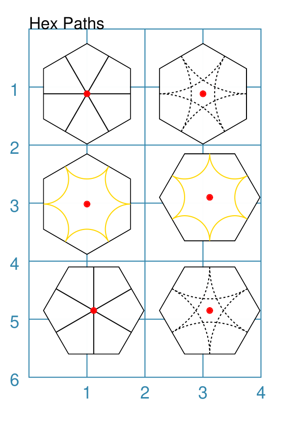
Path: Flat & Pointy
Path lines are drawn between the mid-points of two edges; they can be arcs or straight lines depending on which edges they connnect.
|
This example shows Hexagons constructed using these commands: hxg = Common(
height=1.5, font_size=8,
dot=0.05, dot_stroke="red")
Hexagon(
common=hxg, x=0.25, y=0.25,
orientation="pointy",
paths=["ne sw", "e w", "se nw"])
Hexagon(
common=hxg, x=0.25, y=2.15,
orientation="pointy",
paths=["ne e", "e se", "se sw", "sw w", "w nw", "nw ne"],
paths_stroke="gold")
Hexagon(
common=hxg, x=0.25, y=4.1,
paths=["sw ne", "se nw", "s n"])
Hexagon(
common=hxg, x=2.25, y=4.1,
paths=["s ne", "se sw", "s nw", "nw ne", "n se", "n sw"],
paths_dotted=True)
Hexagon(
common=hxg, x=2.25, y=2.15,
paths=["ne n", "ne se", "se s", "sw s", "sw nw", "nw n"],
paths_stroke="gold")
Hexagon(
common=hxg, x=2.25, y=0.25,
orientation="pointy",
paths=["ne se", "e sw", "se w", "sw nw", "w ne", "nw e"],
paths_dotted=True)
These have the following properties:
The Hexagons with normal line styles have links between opposing edges. The Hexagons with gold colored line have links between adjacent edges. The Hexagons with dotteed line styles have links between edges that are not opposite or adjacent. |
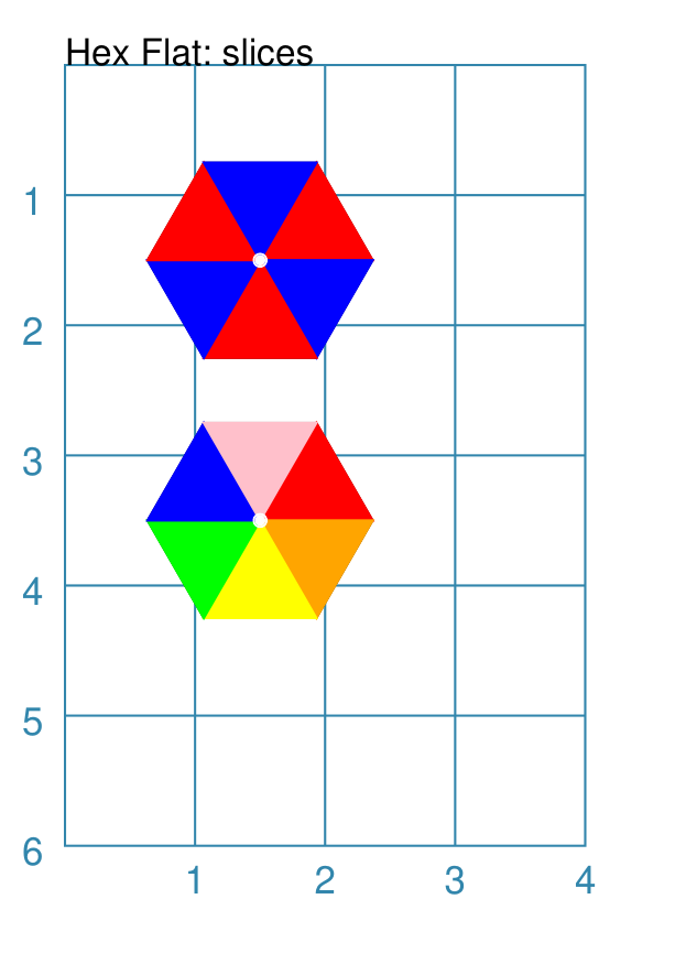
Slices: Flat
Slices are a set of colors that are drawn as triangles inside a a Hexagon in a clockwise direction starting from the “North East”. If there are fewer colors than the six possible triangles, then the colors are repeated, starting from the first one.
|
This example shows Hexagons constructed using these commands: hxg = Common(height=1.5, dot=0.05, dot_stroke="white", font_size=8)
Hexagon(
common=hxg,
cx=1.5, cy=1.5,
slices=['red', 'blue'],
orientation="flat")
Hexagon(
common=hxg, cx=1.5, cy=3.5,
slices=['red', 'orange', 'yellow', 'green', 'blue', 'pink'],
orientation="flat")
These Hexagons all share the following Common properties that differ from the defaults:
Each Hexagon has its own setting for:
|
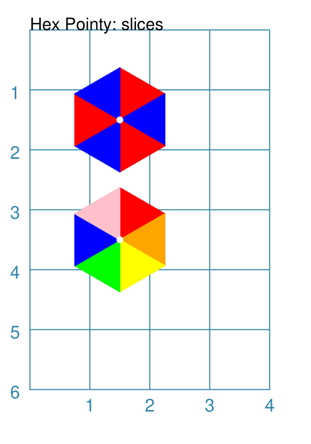
Slices: Pointy
Slices are a set of colors that are drawn as triangles inside a a Hexagon in a clockwise direction starting from the “North East”. If there are fewer colors than the six possible triangles, then the colors are repeated, starting from the first one.
|
This example shows Hexagons constructed using these commands: hxg = Common(
height=1.5,
dot=0.05, dot_stroke="white")
Hexagon(
common=hxg,
cx=1.5, cy=1.5,
slices=['red', 'blue'], orientation="pointy")
Hexagon(
common=hxg,
cx=1.5, cy=3.5,
slices=['red', 'orange', 'yellow', 'green', 'blue', 'pink'],
orientation="pointy")
These Hexagons all share the following Common properties that differ from the defaults:
Each Hexagon has its own setting for:
|
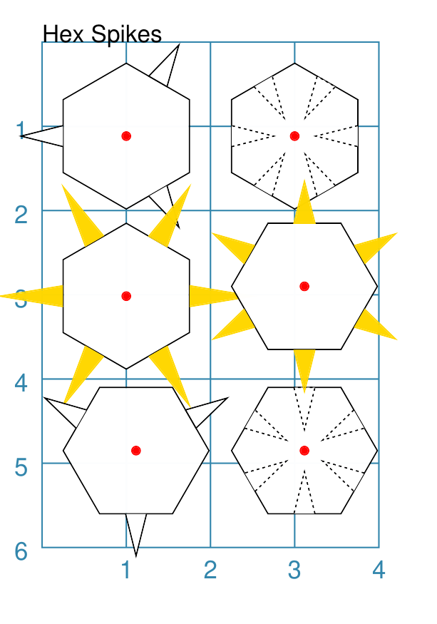
Spikes
Spikes are a set of one or more triangles drawn at the “perbii points” i.e. with the base of the triangles centred on the middle of Hexagon edges.
If the height of the spike is given as a negative number, then the triangle will point to the inside of the Hexagon.
|
This example shows Hexagons constructed using these commands: hxg = Common(
height=1.5,
dot=0.05, dot_stroke="red",
spikes_width=0.25)
Hexagon(
common=hxg, x=0.25, y=0.25,
orientation="pointy",
spikes=["ne", "w", "se"],
spikes_height=0.5)
Hexagon(
common=hxg, x=2.25, y=4.1,
spikes=["s", "sw", "nw", "ne", "se", "n"],
spikes_dotted=True,
spikes_height=-0.5)
Hexagon(
common=hxg, x=2.25, y=0.25,
orientation="pointy",
spikes=["ne", "se", "sw", "w", "nw", "e"],
spikes_height=-0.5,
spikes_dotted=True)
Hexagon(
common=hxg, x=0.25, y=2.15,
orientation="pointy",
spikes=["ne", "se", "sw", "w", "nw", "e"],
spikes_stroke="gold",
spikes_fill="gold")
Hexagon(
common=hxg, x=0.25, y=4.1,
spikes=["ne", "nw", "s"],
spikes_height=0.5)
Hexagon(
common=hxg, x=2.25, y=2.15,
spikes=["s", "sw", "nw", "ne", "se", "n"],
spikes_height=0.5,
spikes_stroke="gold",
spikes_fill="gold")
These Hexagons all share the following Common properties that differ from the defaults:
The directions of all of the spikes are given in list form; but a
string format such as The top- and bottom-left hexagons show typical spikes, each with a
spikes_height of The centre left and right hexagons show spikes with a default height
equal to the hexagon’s edge length. They also have their line and fill
color both set to The top- and bottom-right hexagons show inner-facing spikes, each with a
spikes_height of |
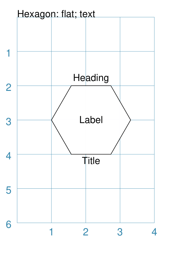
Text: Flat
|
This example shows a Hexagon constructed using this command: Hexagon(
y=2,
height=2,
title="Title",
label="Label",
heading="Heading")
It has the following properties that differ from the defaults:
All of this text is, by default, centred horizontally. Each text item can be further customised in terms of its color, size and font family. The can be done by appending _stroke, _stroke_width, _size and _font respectively to the text type’s name. |
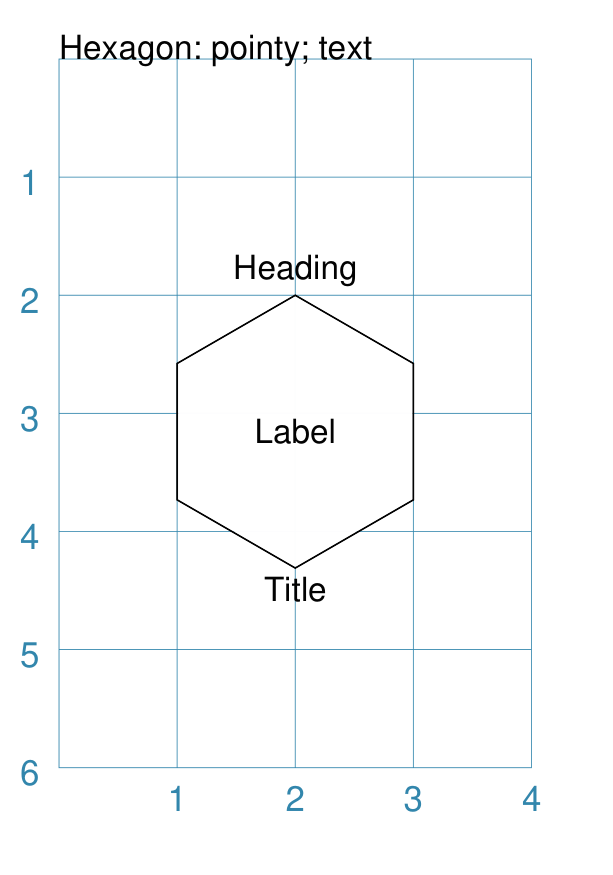
Text: Pointy
|
This example shows a Hexagon constructed using this command: Hexagon(
y=2,
height=2,
orientation='pointy',
title="Title",
label="Label",
heading="Heading")
It has the following properties that differ from the defaults:
All of this text is, by default, centred horizontally. Each text item can be further customised in terms of its color, size and font family. The can be done by appending _stroke, _stroke_width, _size and
_font respectively to the text type’s name. For example, using
|
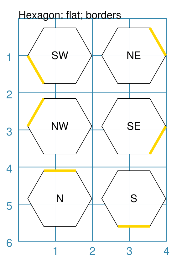
Borders
The Borders property allows for the normal line, that is drawn around a
Hexagon, to be overwritten on specific sides by another type of line.
The Borders property is specified by providing a set of values, which are
comma-separated inside of round brackets, in the following order:
direction - one of (n)orth, (s)outh, (e)ast, (w)est, ne(northeast), se(southeast), nw(northwest), or sw(southwest)
width - the line thickness
color - either a named color or a hexadecimal value
style -
Truemakes it dotted; or a list of values creates dashes
Direction and width are required, but color and style are optional.
One or more border values can be used together with spaces between them
e.g. ne se to draw lines on both northeast and southeast.
Example 1. Flat
|
This example shows hxg = Common(
height=1.5, orientation="flat", font_size=8)
Hexagon(
common=hxg, x=0.25, y=0.25,
borders=('sw', 2, "gold"), label="SW")
Hexagon(
common=hxg, x=0.25, y=2.15,
borders=('nw', 2, "gold"), label="NW")
Hexagon(
common=hxg, x=0.25, y=4.00,
borders=('n', 2, "gold"), label="N")
Hexagon(
common=hxg, x=2.25, y=4.00,
borders=('s', 2, "gold"), label="S")
Hexagon(
common=hxg, x=2.25, y=0.25,
borders=('ne', 2, "gold"), label="NE")
Hexagon(
common=hxg, x=2.25, y=2.15,
borders=('se', 2, "gold"), label="SE")
Each Hexagon has a normal stroke_width as its outline, with a default fill and stroke color of black. For each Hexagon, there is a single thick yellow line on one side set by the direction in borders. |
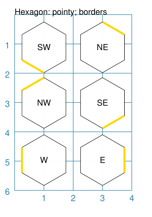
Example 2. Pointy
|
This example shows hxg = Common(
height=1.5, orientation="pointy", font_size=8)
Hexagon(
common=hxg, x=2.25, y=4.00,
common=hxg, x=0.25, y=0.25,
borders=('sw', 2, "gold"), label="SW")
Hexagon(
common=hxg, x=0.25, y=2.15,
borders=('nw', 2, "gold"), label="NW")
Hexagon(
common=hxg, x=0.25, y=4.00,
borders=('w', 2, "gold"), label="W")
Hexagon(
common=hxg, x=2.25, y=4.00,
borders=('e', 2, "gold"), label="E")
Hexagon(
common=hxg, x=2.25, y=0.25,
borders=('ne', 2, "gold"), label="NE")
Hexagon(
common=hxg, x=2.25, y=2.15,
borders=('se', 2, "gold"), label="SE")
Each Hexagon has a normal stroke_width as its outline, with a default fill and stroke color of black. For each Hexagon, there is a single thick yellow line on one side set by the direction in borders. |
Ordering of Properties
There is a default order in which the various properties of a Hexagon are drawn. There are three ways to change this drawing order:
order_first - a list of properties that will be drawn, in the order given in the list, before any others
order_last - a list of properties that will be drawn, in the order given in the list, after any others
order_all - a list of the only properties that will be drawn, in the order given in the list
The available property names, shown in their default order, are:
base - this represents the Hexagon itself
borders
shades
slices
spikes
hatches
links
perbii
paths
radii_shapes
perbii_shapes
centre_shape
centre_shapes
vertex_shapes
dot
cross
text
numbering
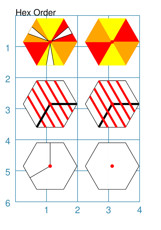
Example 1.
|
This example shows hxg = Common(height=1.5,
dot=0.05, dot_stroke="red")
Hexagon(common=hxg, x=0.25, y=0.1,
slices=['red', 'orange', 'yellow'],
spikes=["ne", "nw", "s"],
spikes_height=-0.7,
spikes_width=0.25)
Hexagon(common=hxg, x=2.25, y=0.1,
slices=['red', 'orange', 'yellow'],
spikes=["ne", "nw", "s"],
spikes_height=-0.7,
spikes_width=0.25
order_first=["spikes"])
Hexagon(common=hxg, x=0.25, y=2.1,
hatches_count=5, hatches_stroke="red",
hatches_stroke_width=2, hatches='nw',
radii='sw e',
radii_stroke_width=2)
Hexagon(common=hxg, x=2.25, y=2.1,
hatches_count=5, hatches_stroke="red",
hatches_stroke_width=2, hatches='nw',
radii='sw e',
radii_stroke_width=2,
order_last=["hatcheses"])
Hexagon(common=hxg, x=0.25, y=4.1,
perbii='sw n')
Hexagon(common=hxg, x=2.25, y=4.1,
perbii='sw n',
order_all=["base", "dot"])
The top-most pair of Hexagons show how changing the order_first property means that the spikes are not visible because they are drawn before the slices (which overwrite them). The middle pair of Hexagons show how changing the order_last property means that hatches are drawn after the radii, instead of before. The lower-most pair of Hexagons show how setting the order_all property means that only the Hexagon and the centre Dot will drawn, and not the perbii. |
Circle
A Circle is a very common shape in many designs; it provides a number of ways that it can be customised.
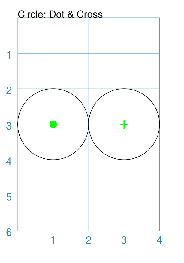
Dot & Cross
|
This example shows Circles constructed using these commands: Circle(
cx=1, cy=3, radius=1,
dot=0.1, dot_stroke="green")
Circle(
cx=3, cy=3, radius=1,
cross=0.25, cross_stroke="green",
cross_stroke_width=1)
These Circles have properties set as follows:
|
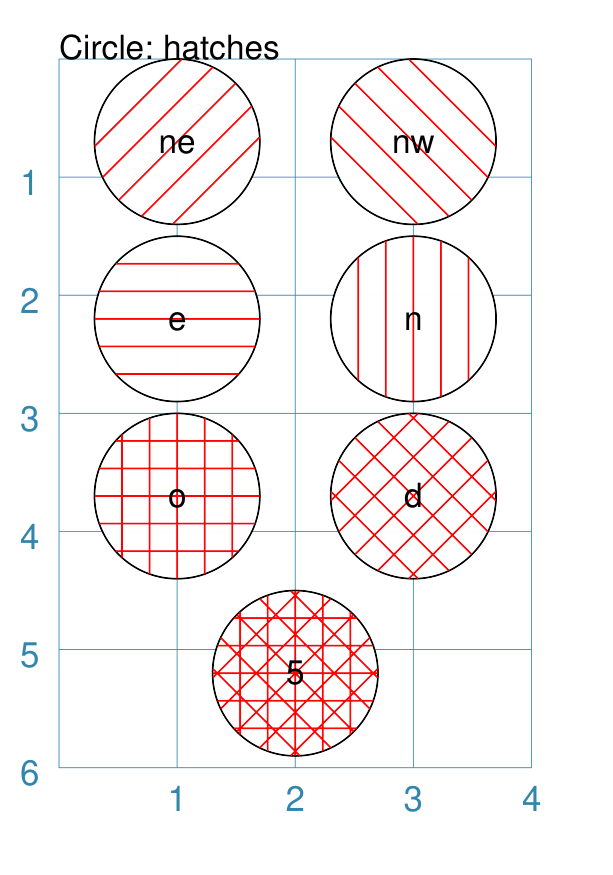
Hatches
Hatches are a set of parallel lines that are drawn, in a specified direction, across the Circle from one opposing side to another in a vertical, horizontal or diagonal direction. Hatches are equally spaced across the diameter of the Circle.
|
This example shows Circles constructed using these commands: htc = Common(
radius=0.7,
hatches_count=5,
hatches_stroke="red")
Circle(
common=htc, cx=2, cy=5.2,
label='5')
Circle(
common=htc, cx=1, cy=3.7,
hatches='o', label='o')
Circle(
common=htc, cx=3, cy=3.7,
hatches='d', label='d')
Circle(
common=htc, cx=1, cy=2.2,
hatches='e', label='e')
Circle(
common=htc, cx=3, cy=2.2,
hatches='n', label='n')
Circle(
common=htc, cx=1, cy=0.7,
hatches='ne', label='ne')
Circle(
common=htc, cx=3, cy=0.7,
hatches='nw', label='nw')
These Circles all share the following Common properties that differ from the defaults:
Each Circle has its own setting for:
|
Hatches: Variable
As described in section on Hatches, these are normally spaced equally across the height or width of the Circle.
However it is possible to vary the number of hatch lines for any direction, or set of directions, by changing the setting for the hatches property.
This is illustrated in the example below.
|
This example shows a Circle constructed using these commands: Circle(
common=htc,
hatches=[('e', 3), ('d', 5)],
hatches_stroke_width=0.5,
hatches_stroke="red")
While other settings are similar to the previous example, in this
case the hatches property is in a list form, as shown by the square
brackets from
In this case, there are 3 lines in the |
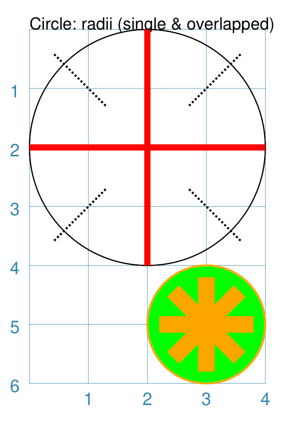
Radii
Radii are like spokes of a bicycle wheel; they are drawn from the centre of a Circle towards its circumference.
|
This example shows Circles constructed using these commands: Circle(x=0, y=0, radius=2,
fill=None,
radii=[45,135,225,315],
radii_stroke_width=1,
radii_dotted=True,
radii_offset=1,
radii_length=1.25)
Circle(x=0, y=0, radius=2,
fill=None,
radii=[0,90,180,270],
radii_stroke_width=3,
radii_stroke="red")
Circle(cx=3, cy=5, radius=1,
fill="green",
stroke="orange", stroke_width=1,
radii=[0,90,180,270,45,135,225,315],
radii_stroke_width=8,
radii_stroke="orange",
radii_length=0.8)
The top two circles are drawn at the same location with the same
basic properties; with their fill set to These Circles also have some of the following properties, which demonstrate how radii can be set and customised:
|
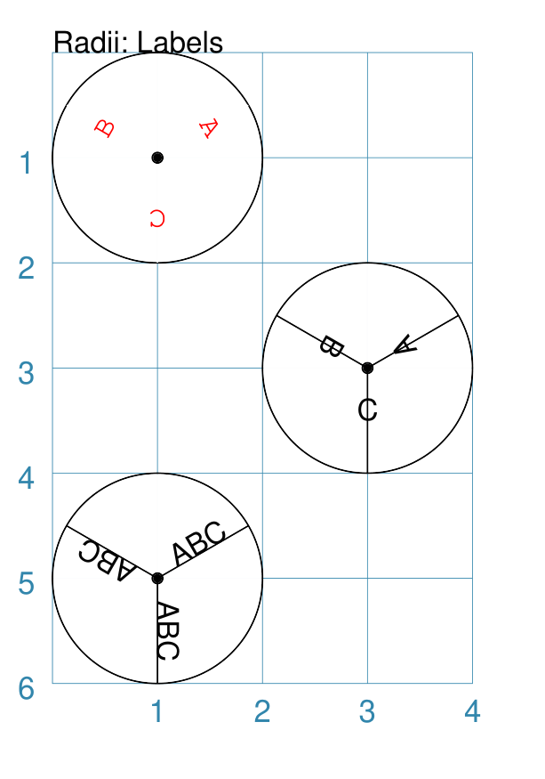
Radii - Labels
Radii labels are text lines linked to one or more radii. Text can be repeated or unique. It can also be rotated — relative to the radius line it is on — and styled with stroke color, size, and face.
|
This example shows Circles constructed using these commands: Circle(cx=1, cy=1, radius=1,
radii=[30, 150, 270],
radii_stroke="white",
radii_labels=["A", "B", "C"],
radii_labels_rotation=270,
radii_labels_stroke="red",
radii_labels_font="Courier",
dot=0.05)
Circle(cx=3, cy=3, radius=1,
radii=[30, 150, 270],
radii_labels="A,B,C",
radii_labels_rotation=90,
dot=0.05)
Circle(cx=1, cy=5, radius=1,
radii=[30, 150, 270],
radii_labels="ABC",
dot=0.05)
Apart from the radii lines themselves, the labels’ properties can be set:
The top-most example shows how text strings are created with a list. The middle example shows how the text string is split using commas; this results in a list whose members are used to create the labels. The lower-most example shows how the same text is repeated for all radii. The top example also shows how text is rotated and styled. The radii lines’ stroke color is set to match the circle fill, thereby making it “invisible”. The label rotation is relative to its upright position on the line; so 90° turns the text to the left and onto its “side”, as shown in the middle example. |
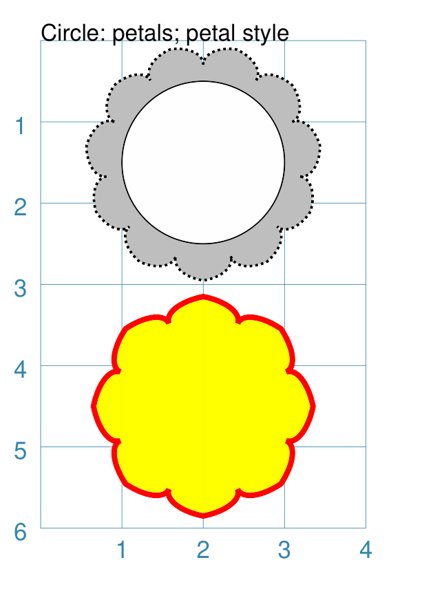
Petals - petal
Petals are projecting shapes drawn from the circumference of a Circle outwards at regular intervals. They are typically used to create a “flower” or “sun” effect.
|
This example shows Circles constructed using these commands: Circle(cx=2, cy=1.5, radius=1,
petals=11,
petals_style="petal",
petals_offset=0.2,
petals_stroke_width=1,
petals_dotted=1,
petals_height=0.25,
petals_fill="gray")
Circle(cx=2, cy=4.5, radius=1,
fill_stroke="yellow",
petals=8,
petals_style="p",
petals_offset=0.1,
petals_stroke_width=2,
petals_height=0.25,
petals_stroke="red",
petals_fill="yellow")
These Circles have the following properties:
|
Petals - triangle
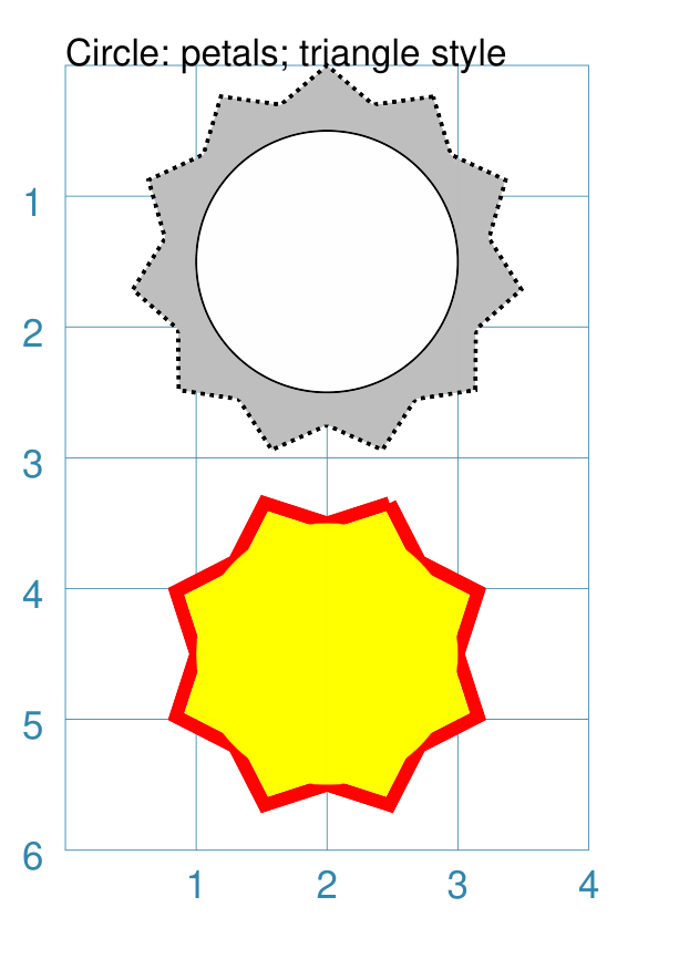
Petals are projecting shapes drawn from the circumference of a Circle outwards at regular intervals. They are typically used to create a “flower” or “sun” effect.
|
This example shows Circles constructed using these commands: Circle(cx=2, cy=1.5, radius=1,
petals=11,
petals_offset=0.25,
petals_stroke_width=1,
petals_dotted=True,
petals_height=0.25,
petals_fill="grey")
Circle(cx=2, cy=4.5, radius=1,
stroke=None, fill=None,
petals=8,
petals_stroke_width=3,
petals_height=0.25,
petals_stroke="red",
petals_fill="yellow")
These Circles have the following properties:
Note that these petals have a default petals_style of
|
Petals - sun
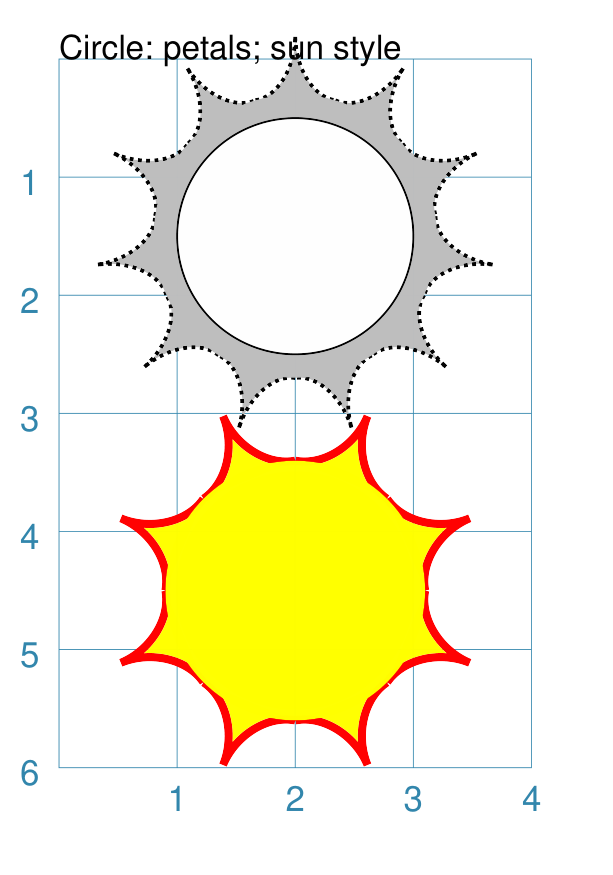
Petals are projecting shapes drawn from the circumference of a Circle outwards at regular intervals. They are typically used to create a “flower” or “sun” effect.
|
This example shows Circles constructed using these commands: Circle(cx=2, cy=1.5, radius=1,
petals=11,
petals_style="sun",
petals_offset=0.25,
petals_stroke_width=1,
petals_dotted=True,
petals_height=0.5,
petals_fill="grey")
Circle(cx=2, cy=4.5, radius=1,
stroke=None, fill=None,
petals=8,
petals_style="s",
petals_stroke_width=3,
petals_height=0.5,
petals_stroke="red",
petals_fill="yellow")
These Circles have the following properties:
Note that these petals have the petals_style of |
Slices
The slices property enables the Circle to be filled with colored pie-shaped wedges.
These are the relevant properties that can be set:
slices - this is a list of colors (named or hexadecimal); if
Noneis used then no slice will be drawn in that positionslices_fractions - this is the “length” of the slices; if not specified, then by default all slices will have their fraction set to
1meaning they are equal to the radius of the circle — values smaller than1will result in them being drawn inside the circle and values larger than1will result in them extending outside of the circleslices_angles - this is the “width” of the slices; if not specified, then by default all slices will be of equally-sized angles and will extend from the centre to the full circumference of the circle
slices_transparency - the higher the value (on a scale of 0 to 100), the more “see through” the fill of the slices will be
Both the list of slice_fractions and slice_angles must be of equal length to the slice list.
Note
Slices are drawn after the circle has been drawn, and so may obscure the stroke outline, fill color and other properties of the circle.
|
This example shows Circles constructed using the commands: Circle(cx=1, cy=1, radius=1,
slices=["red", "gold", "aqua"],
dot=0.05)
Circle(cx=2, cy=3, radius=1,
slices=["red", None, "red", None, "red", None],
dot=0.05)
Circle(cx=3, cy=5, radius=1,
slices=["red", "gold", "aqua", "red", "gold", "aqua"],
rotation=30,
dot=0.05)
Circle(cx=3, cy=1, radius=1,
slices=["black", "grey", "silver"],
slices_fractions=[0.33, 0.75, 0.5])
Circle(cx=1, cy=5, radius=1, fill="gold",
slices=["black", None, "grey", "silver"],
slices_fractions=[0.33, None, 1.5, 0.75],
slices_angles=[60, 45, 45, 120])
The top-left example shows the minimum required; the slices property is
a list of colors ( The middle example shows what happens when the slices property includes
the The lower-right example shows what happens when the rotation property is also set; the slices start position is offset that many degrees anti-clockwise from the 0° (east) position. The top-right example shows the use of the slices_fractions property;
because values are less than The bottom-left example show the use of the slices_fractions property
and what happens when the slices property and the matching
slices_fractions property both include the Note All slice lines are drawn with the slices_stroke color, which defaults to the slice color itself. |
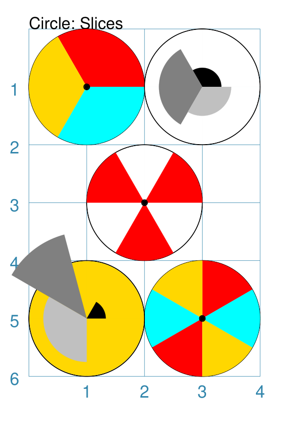
Nested
The nested property enables the Circle to be filled with a series of concentric circles.
|
This example shows Circles constructed using the commands: Circle(
cx=1, cy=1, radius=1,
nested=2)
Circle(
cx=2, cy=3, radius=1,
nested=[0.8, 0.1, 0.4])
Circle(
cx=3, cy=5, radius=1,
nested=4,
dotted=True,
stroke="red",
fill="yellow")
The nested property can either be a single whole number or a list of fractional numbers. Each fractional number in the list indicates a Circle to be drawn at
a distance corresponding to the fraction of the circle’s radius.
For example, if circle’s radius is Note All nested Circles are drawn with the same line and fill properties as the Circle shape to which they are part of. For more control over such features, rather use the centre_shape property instead, as this will permit construction of a circle with any/all properties being set. |
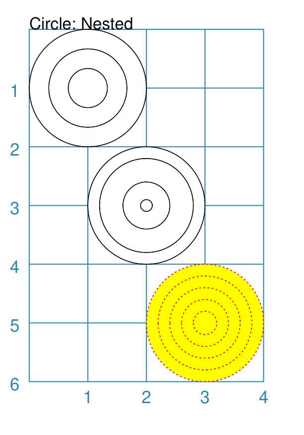
Ordering of Properties
There is a default order in which the various properties of a Circle are drawn. There are three ways to change this drawing order:
order_first - a list of properties that will be drawn, in the order given in the list, before any others
order_last - a list of properties that will be drawn, in the order given in the list, after any others
order_all - a list of the only properties that will be drawn, in the order given in the list
The available property names, shown in their default order, are:
petals
base - this represents the Circle itself
nested
slices
hatches
radii
radii_shapes
centre_shape
centre_shapes
dot
cross
text
Triangle
Triangle overview
A triangle is a three-sided polygon. It can have uniform sides, in which case it is an equilateral triangle — the default; two sides of matching length, in which case it is an isosceles triangle; or all sides of unequal length, in which case it is an irregular triangle.
A triangle is considered to have three vertices located using the
following compass directions; n (north), sw (south-west), and se
(south-east). Similarly, the three sides are located at ne (north-east),
nw (north-west), and s (south).
A triangle has a centroid, or “center of mass”, which is the point where the three lines from the vertices to the midpoints of the opposite sides intersect. It is used as the point around which all elements of triangle can be rotated.
Triangle construction
The starting point for drawing a triangle is the sw vertice. The s
line is then drawn, usually in the e direction, followed by the ne
line, and finally the ne.
Note
Unlike most other shapes, the Triangle’s x and y positions are NOT at the top-left “corner”. This breaks with convention, but the concept of such a corner just does not seem to work in this case.
All triangles require the starting point to be set, if different from the
default of 1 for both the x and y positions.
A triangle’s drawing can be affected by its pivot which is an angle used to
alter the direction of the bottom edge — the s line. By default this
line is drawn in the eastwards direction, i.e. a pivot of 0°, but if
set will cause that line to be rotated anti-clockwise around the sw vertex.
Equilateral triangles
Equilateral triangles are the simplest to construct. Apart from the starting point, all that is required is the length of the side to be set. All sides share the same length.
Because protograf uses a default value of 1 for the side
property, an equilateral triangle is the default one that will be constructed
unless more properties are set. See Example 1. Default Triangle.
Equilateral triangles can also be constructed using their centroid position, instead of the usual x and y positions. See Example 2. Custom Equilateral
Note
An Equilateral triangle constructed via its centroid position cannot also have a value set for pivot. This is because this setting would effectively be acting in the same way as the rotation.
Isosceles triangles
Isosceles triangles require both the length of the bottom edge to be set — via the side property — as well as the height. The other two sides will be equal in length and calculated from the side and height properties. See Example 3. Custom Isosceles.
Irregular triangles
Irregular triangles are the most complex to construct. There are a number of options to do so.
Set the values for side2 and side3. Their total must exceed the value set for side.
Set the values for side2 and angle. This will draw the second line, of length side2, at the given angle relative to side.
Set the value for side2. This will set the angle to 90° and cause a right-angled triangle to be drawn.
For illustrations of these construction options, see Example 4a. Custom Irregular I and Example 4b. Custom Irregular II.
Triangle construction examples
Example 1. Default Triangle
|
This example shows the Triangle constructed using the command with only defaults: Triangle()
It has the following properties based on the defaults:
|
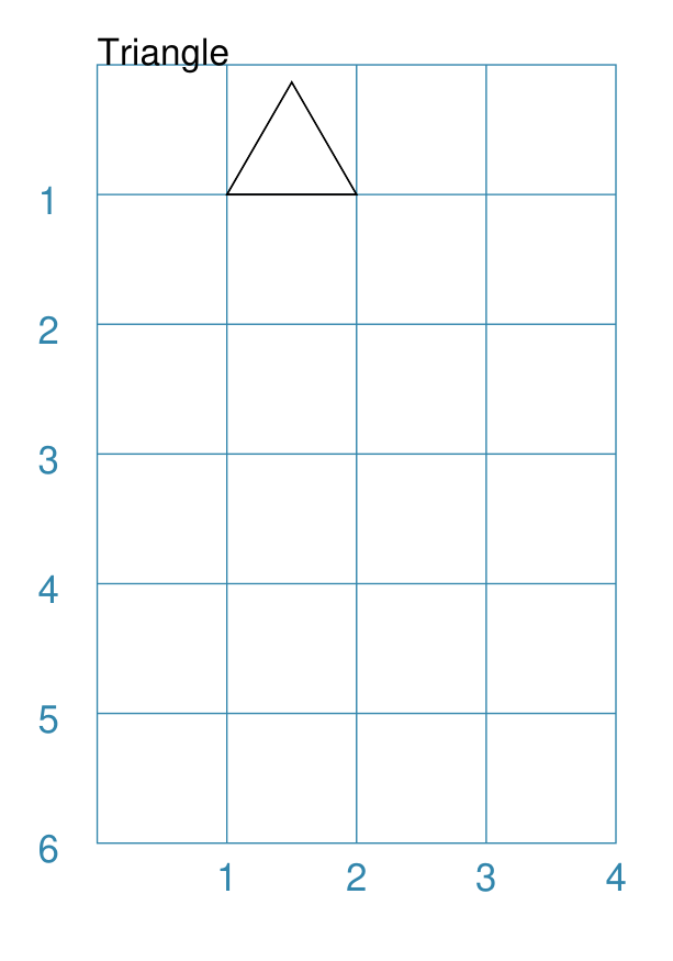
Example 2. Custom Equilateral
|
This example shows the Triangle constructed using the command as follows: Triangle(
cx=2, cy=3,
side=3,
stroke_width=1,
fill="gold",
title="Equilateral")
It has the following properties:
|
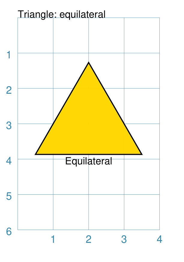
Example 3. Custom Isosceles
|
This example shows the Triangle constructed using the command as follows: Triangle(
x=0.5, y=5,
side=3, height=4,
stroke_width=1,
fill="lime",
title="Isosceles")
It has the following properties:
|
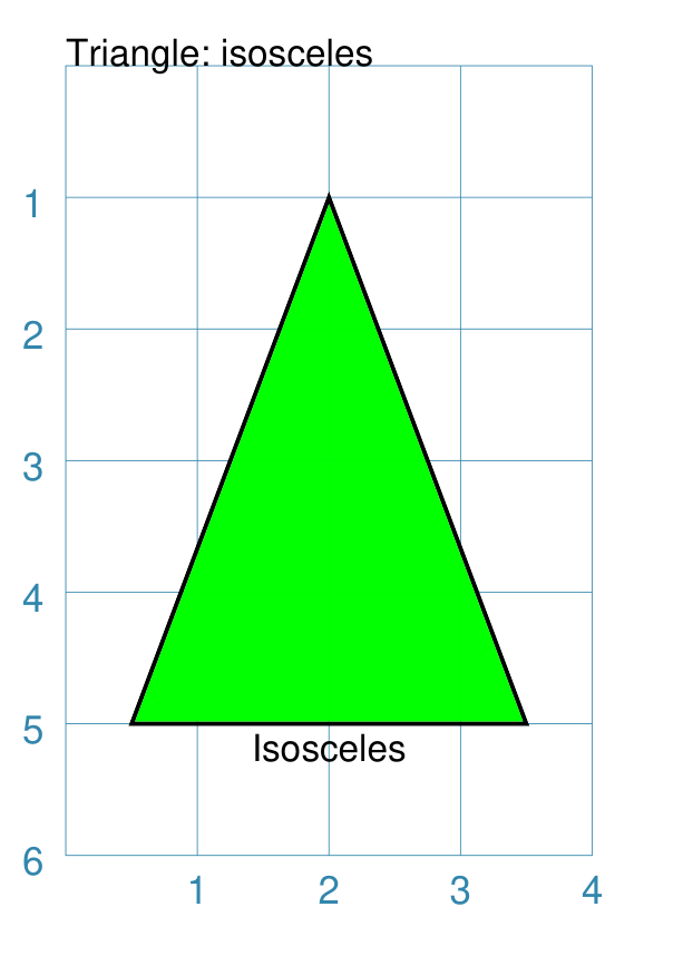
Example 4a. Custom Irregular I
|
This example shows the Triangle constructed using the command as follows: Triangle(
x=1, y=4,
side=3, side2=4.5, side3=2.5,
stroke_width=1,
fill="tomato",
title="Irregular")
It has the following properties:
|
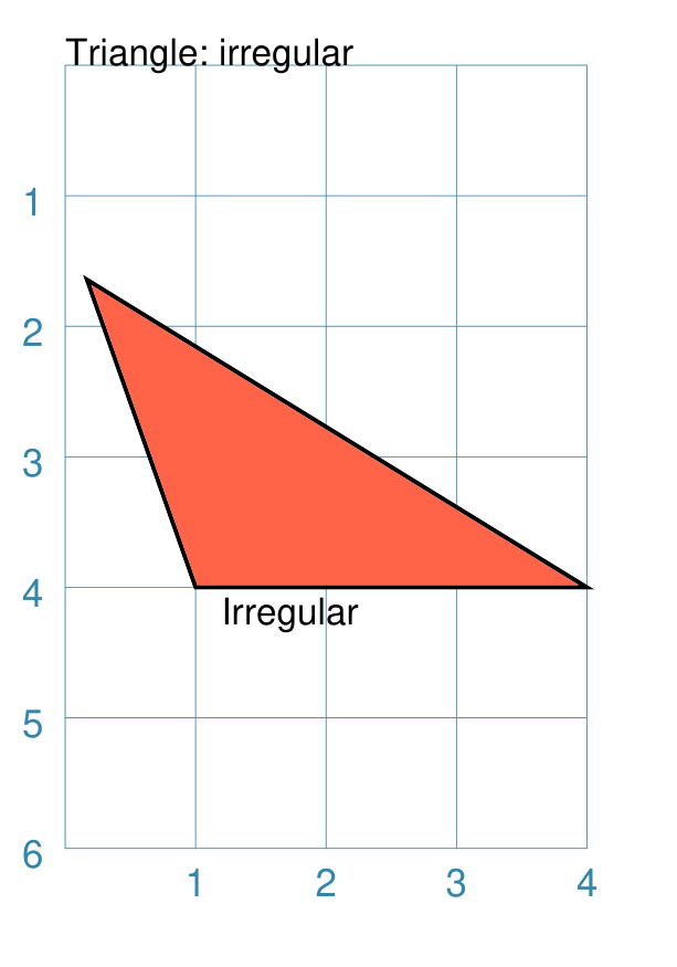
Example 4b. Custom Irregular II
|
This example shows the Triangle constructed using the command as follows: Triangle(
x=0, y=2,
side=1.5, side2=1.75, side3=2.55,
stroke_width=0.5,
dot=0.06,
title="3xsides",
title_size=7)
Triangle(
x=2, y=2,
side=1.5, side2=1.75, side3=2.55,
pivot=30,
stroke_width=0.5,
dot=0.06,
title="pivot:30",
title_size=7)
Triangle(
x=0, y=4,
side=1.5, side2=1.75, angle=115,
stroke_width=0.5,
dot=0.06,
title="2xsides; 115",
title_size=7)
Triangle(
x=2, y=4,
side=2, side2=1.5,
stroke_width=0.5,
dot=0.06,
title="2xsides; rightangle",
title_size=7)
Triangle(
x=0, y=6,
side=1.5, side2=1.5, side3=1.5,
pivot=30,
stroke_width=0.5,
dot=0.06,
title="equi; pivot:45",
title_size=7)
Triangle(
x=3.5, y=6,
side=1.25, side2=1.75, side3=1.75,
pivot=90,
stroke_width=0.5,
dot=0.06,
title="iso; pivot:90",
title_size=7)
These examples illustrate the various construction techniques. The lower two examples show how the other types of triangles can also be constructed via setting the appropriate properties of an irregular triangle. |
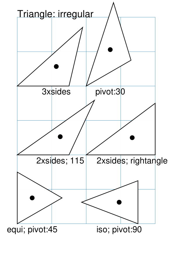
Triangle customisation
There are a number of ways that a Triangle can be customised.
Cross and Dot
A cross or a dot are symbols that are used to mark the centroid of the Triangle. They are usually the last elements that are drawn.
Example 5. Triangle: Cross & Dot
|
This example shows Triangles constructed using the commands: Triangle(
x=1, y=2, side=2,
stroke_width=1,
dot=.05,
cross=0.33, cross_stroke="red",
cross_stroke_width=1,
title="Equilateral")
Triangle(
x=1, y=4,
side=2, height=1.25,
stroke_width=1,
dot=.05,
cross=0.33, cross_stroke="red",
cross_stroke_width=1,
title="Isosceles")
Triangle(
x=1.25, y=5.5,
side=2, side2=2.5, side3=1.25,
stroke_width=1,
dot=.05,
cross=0.33, cross_stroke="red",
cross_stroke_width=1,
title="Irregular")
The top example shows a dot, superimposed with a red cross, at the centroid position of an equilateral Triangle. The middle example shows a dot, superimposed with a red cross, at the centroid position of an isosceles Triangle. The lower example shows a dot, superimposed with a red cross, at the centroid position of an irregular Triangle. |
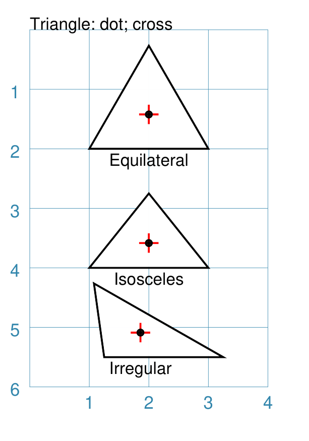
Hatches
Hatches are a set of parallel lines that are drawn, in a specified direction, across the Triangle from one opposing side to another.
Example 6a. Triangle: Hatches
These examples show hatch starting points that are equally spaced across each of the sides of the Triangle.
|
This example shows the shape constructed using the command with the various properties. Triangle(
x=1, y=2, side=2,
hatches_count=5,
hatches_stroke="red",
title="Equilateral")
Triangle(
x=1, y=4,
side=2, height=1.25,
hatches_count=5,
hatches_stroke="red",
title="Isosceles")
Triangle(
x=1.25, y=5.5,
side=2, side2=2.5, side3=1.25,
hatches_count=5,
hatches_stroke="red",
title="Irregular")
The top example shows hatches constructed in all directions for a equilateral Triangle. The middle example shows hatches constructed in all directions for a isosceles Triangle. The lower example shows hatches constructed in all directions for a irregular Triangle. |
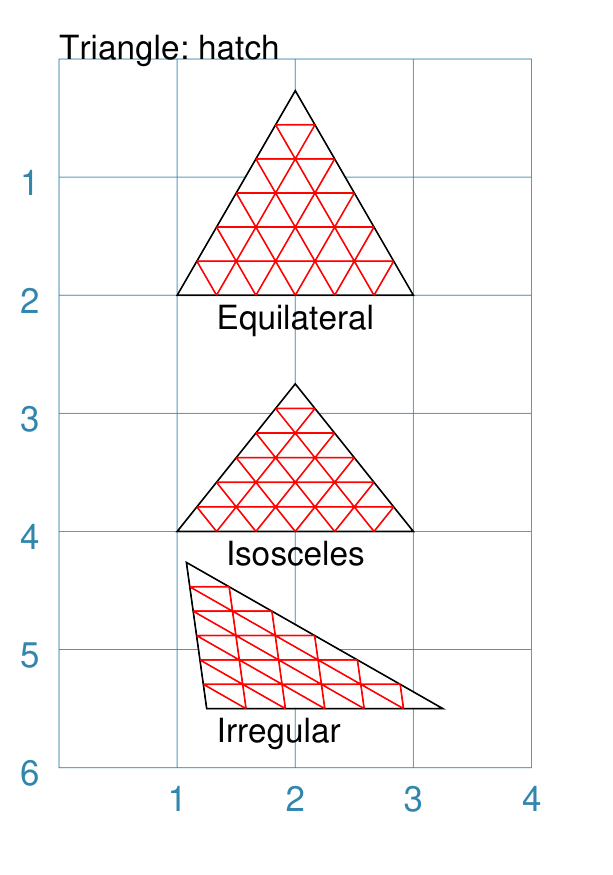
Example 6b. Triangle: Hatches - Variable
As described in Example 6a above, hatches are normally spaced equally across the sides of the Triangle.
However it is possible to vary the number of hatch lines for any direction, or set of directions, by changing the setting for the hatches property.
|
This example shows the shape constructed using the command with the various properties. Triangle(
x=1, y=3, side=2,
hatches=[('e', 3), ('se', 6)],
hatches_stroke_width=0.5,
hatches_stroke="red")
While other settings are similar to the previous example, in this
case the hatches property is in a list form, as shown by the square
brackets from
In this case, there are 3 lines in the |
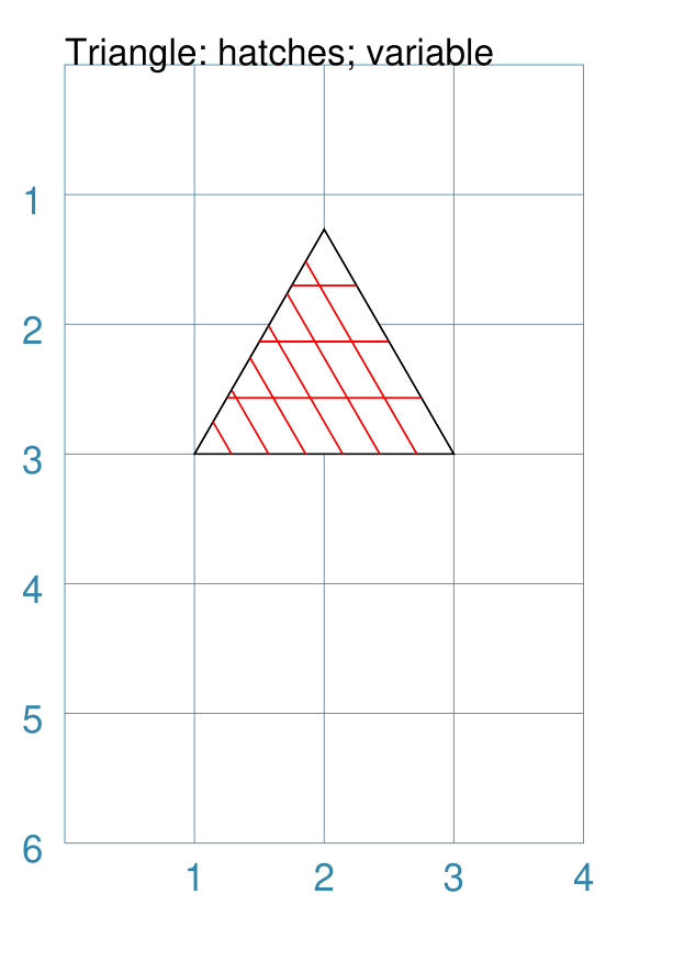
Perbii
“Perbis” is a shortcut name for “perpendicular bisector”; and perbii is the the plural. These lines are drawn from the centroid of a Triangle towards the mid-points of its edges.
Example 7. Triangle: Perbii
|
This example shows triangles constructed using these commands: a_dot = dot(dot_width=4, fill="white")
Triangle(
cx=2, cy=3,
side=1.5,
perbii="s ne nw",
centre_shapes=[(a_dot)],
title="perbii",
fill="gold")
All examples share a common small circle, or The top example shows perbii constructed in all directions for an equilateral Triangle. The middle example shows perbii constructed in all directions for an isosceles Triangle. The lower example shows perbii constructed in all directions for an irregular Triangle. |
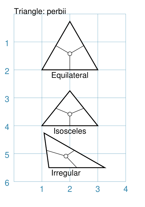
Rotation
Rotation takes place in anti-clockwise direction, from the horizontal, around the centroid of the Triangle.
Example 8. Triangle: Rotation
|
This example shows Triangles constructed using these commands: Triangle(
x=1, y=2, side=2,
stroke_width=1,
rotation=45,
dot=.05,
title="Equilateral")
Triangle(
x=1, y=4,
side=2, height=1.25,
stroke_width=1,
rotation=45,
dot=.05,
title="Isosceles")
Triangle(
x=1.25, y=5.5,
side=2, side2=2.5, side3=1.25,
stroke_width=1,
rotation=45,
dot=.05,
title="Irregular")
The top example shows rotation of 45° anti-clockwise for an equilateral Triangle. The middle example shows rotation of 45° anti-clockwise for an isosceles Triangle. The lower example shows rotation of 45° anti-clockwise for an irregular Triangle. |
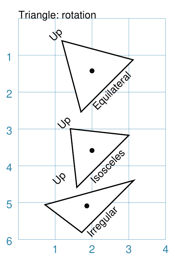
Radii
Radii are the lines drawn from the centroid of a Triangle towards its vertices.
Example 9. Triangle: Radii
|
This example shows Triangles constructed using these commands: a_dot = dot(dot_width=4, fill="white")
Triangle(
x=1, y=2, side=2,
stroke_width=1,
radii="n se sw",
centre_shapes=[(a_dot)],
title="Equilateral")
Triangle(
x=1, y=4,
side=2, height=1.25,
stroke_width=1,
radii="n se sw",
centre_shapes=[(a_dot)],
title="Isosceles")
Triangle(
x=1.25, y=5.5,
side=2, side2=2.5, side3=1.25,
stroke_width=1,
radii="n se sw",
centre_shapes=[(a_dot)],
title="Irregular")
All examples share a common small circle, or The top example shows radii constructed in all directions for an equilateral Triangle. The middle example shows radii constructed in all directions for an isosceles Triangle. The lower example shows radii constructed in all directions for an irregular Triangle. |
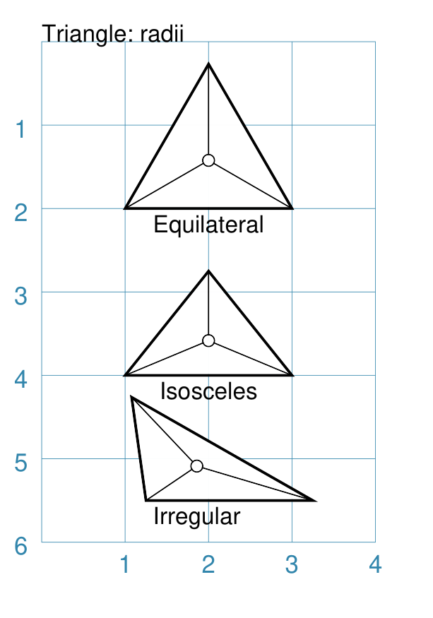
Slices
Slices are a set of colors that are drawn as triangles inside an
Triangle in a clockwise direction starting from the “north-east” (ne)
vertex.
If there are fewer colors than the three possible triangles, then the colors are repeated, starting from the first one.
The term None can be used to skip drawing of a slice i.e. the normal
fill color of the Triangle will appear in that area.
Example 10. Triangle: Slices
|
This example shows triangles constructed using these commands: a_dot = dot(dot_width=4, fill="white")
Triangle(
x=1, y=2, side=2,
stroke_width=1,
slices=["tomato", "gold", "lime"],
centre_shapes=[(a_dot)],
title="Equilateral")
Triangle(
x=1, y=4,
side=2, height=1.25,
stroke_width=1,
slices=["tomato", "gold", "lime"],
centre_shapes=[(a_dot)],
title="Isosceles")
Triangle(
x=1.25, y=5.5,
side=2, side2=2.5, side3=1.25,
stroke_width=1,
slices=["tomato", "gold", "lime"],
centre_shapes=[(a_dot)],
title="Irregular")
All examples share a common small circle, or The top example shows slices constructed in three different colors for an equilateral Triangle. The middle example shows slices constructed in three different colors for an isosceles Triangle. The lower example shows slices constructed in three different colors for an irregular Triangle. |
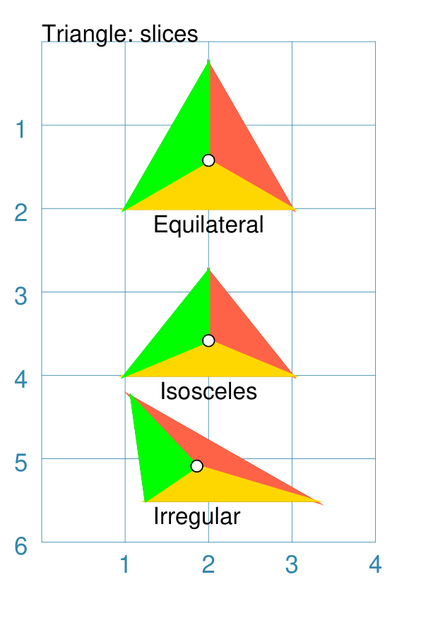
Pivot
A pivot is the number of degrees, in an anti-clockwise direction from
the east, by which a Triangle is rotated around its “south-west” (sw)
vertex.
Note
This type of rotation does not affect the drawing of the text or cross for the Triangle; for this to change direction, the Triangle must be rotated.
Example 11. Triangle: Pivot
|
This example shows triangles constructed using these commands: Triangle(
x=1, y=2, side=2,
stroke_width=1,
pivot=30,
dot=.05,
title="Equilateral")
Triangle(
x=1, y=4,
side=2, height=1.25,
stroke_width=1,
pivot=30,
dot=.05,
title="Isosceles")
Triangle(
x=1.25, y=5.5,
side=2, side2=2.5, side3=1.25,
stroke_width=1,
pivot=30,
dot=.05,
title="Irregular")
All examples share a common small circle, drawn at their centroid via the dot property. The top example shows a pivot of 30° around the south-west vertex for an equilateral Triangle. The middle example shows a pivot of 30° around the south-west vertex for an isosceles Triangle. The lower example shows a pivot of 30° around the south-west vertex for an irregular Triangle. |
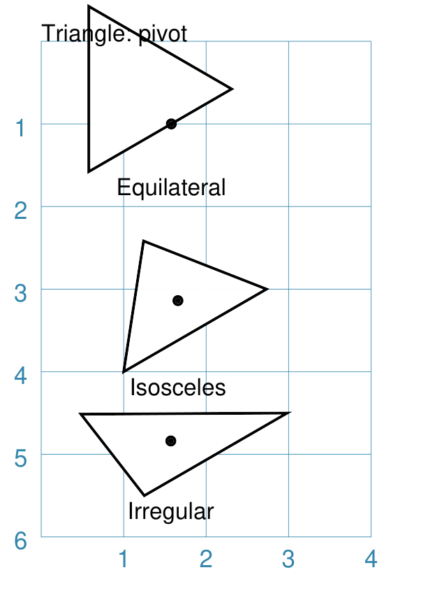
Triangle ordering of properties
There is a default order in which the various properties of a Triangle are drawn. There are three ways to change this drawing order:
order_first - a list of properties that will be drawn, in the order given in the list, before any others
order_last - a list of properties that will be drawn, in the order given in the list, after any others
order_all - a list of the only properties that will be drawn, in the order given in the list
The available property names, shown in their default order, are:
base - this represents the Triangle itself
slices
hatches
perbii
radii
centre_shape
centre_shapes
vertex_shapes
cross
dot
text